Jekyll2026-05-13T22:20:59+00:00http://valhovey.github.io/blog/feed.xmlVal HoveyHere you will find occasional musings I have on math, science, and other things.<br><a target="_blank" rel="me" href="https://valhovey.github.io">Portfolio</a><br><a target="_blank" rel="me" href="https://mathstodon.xyz/@speleo">Mathstodon</a>Star Color and the Evolution of Space on the Screen2026-05-12T00:00:00+00:002026-05-12T00:00:00+00:00http://valhovey.github.io/blog/star-color-and-the-evolution-of-space-on-the-screen
I’m still processing everything I experienced watching the theatrical release of Project Hail Mary. There are seemingly innumerable ways a big screen adaptation of Andy Weir’s masterpiece of a novel could have gone wrong, and yet they managed to succeed in all of them, including ones I did not even consider. For me, the most marvelous result of the film adaptation is that they somehow matched Weir’s diligent and obsessive scientific accuracy in their visual approach to portraying space. I do astrophotography and spend hours on each of my images obsessing over the process and I still get details wrong all of the time. I don’t think it is a controversial take that Project Hail Mary succeeded in rendering space more accurately than any movie before it. I’d like to focus on just one element of this picture: star color and the Milky Way.
Star Color
You would be forgiven if you thought that most stars were just monochromatic point lights suspended in an inky black abyss; this is how space is usually portrayed in science fiction and visual media. Stars, in fact, are brilliantly diverse ranging from deep red to saturated blue. Being black body radiators, the chromaticity of stars lie on a curve called the Planckian Locus. This is the source of the “color temperature” concept advertised on indoor lighting and used in photography. If you plot the luminosity against the effective temperature for stars you reveal a distinct structure that elucidates their lifecycle: this is called the Hertzsprung-Russell Diagram. Most stars lie along the main sequence, but depending on their mass they can end up anywhere from a white dwarf to a Red Supergiant.
Wherever you look in the sky you will find a great diversity of stars of all colors. Why then do they seem to be mostly monochromatic when we look at them from a dark sky? The answer lies in our biology. Our retinas that render the world around us to our vision contain two classes of photoreceptors: cones and rods. Cones are responsible for color vision in the day, and rods allow us to see in low light. Unlike cones, rods trade color response for high sensitivity. As a result, dark vision is generally monochromatic. Cameras offer us an enhanced view of the night sky revealing the true color of space, and with longer exposures we learn that space itself is far from empty.
M53, a globular cluster in the Coma Berenices constellation. These dense clusters of stars are some of the oldest objects in the universe. (credit)
The Iris Nebula in Cepheus, a region of the vast galactic Integrated Flux Nebula that sits above our position on the galactic plane. This region of space is illuminated by the blazing light of a blue star. (credit)
Perhaps one of the most beautiful examples of star color in our night sky is the core of our Milky Way. In the Summer in the Northern hemisphere and in the Winter for the Southern hemisphere the core of our galaxy rises overhead at night and reveals an incomprehensible density of gold dust stars, interstellar dust, and vibrant nebulae.
I took this image on a backpacking trip in Utah in early Summer. The seeing that night was good enough to see detail in the dust lanes in the Milky Way and for this one minute exposure to reveal the golden color and even the Lagoon, Trifid, and Eagle nebulae looking into the core of our galaxy.
This image comes from the City of Rocks in Idaho, a beautiful natural preserve where you can go to appreciate the night sky unimpeded by the light pollution of large cities. To the right of the core of the Milky Way you can see the Rho Ophiuchi Cloud Complex containing the intensely orange star Antares and a region of dark dust that will show up even with phone photography.
Factors like light pollution, sky glow, zodiacal light (the glow of dust on the plane of our solar system), and the chromatic aberration of the lens will influence the colors rendered in many captures of the Milky Way. This has unfortunately produced a public perception of the Milky Way as being purple, green, blue, or even monochromatic. I’ve done a fair amount of color correction to help render the accurate colors of the sky in these images, but there are still some problems (you can notice the blue/purple stars in the top of the second image). Even with these smaller details, these images render the color of our sky far more honestly than all media I have seen up until this point in my life.
The Sky in Media
Red Dead Redemption 2, while having perhaps the most accurate night sky box of any video game yet produced, still demonstrates a common error of portraying the Milky Way as brown with monochromatic stars. Another common error in artistically rendering the night sky also involves portraying the dense galactic core as a blob and bright stars as a separate foreground element.
Interstellar was a monumental work in science fiction but often portrays space as empty with a dearth of stars. Astrophotography is featured in the film, but often with contrast so intense that backgrounds are totally black and the color is all but gone in any of the space backgrounds.
The Martian also sadly portrays space as dark and empty, despite having an abundance of scientific accuracy in other parts of the film.
A New Frontier
I want to focus on one scene in Project Hail Mary, which fortunately avoids spoilers as it takes place in the first five minutes of the film. Grace wakes up aboard the Hail Mary from a coma with no memory of how he got here and quickly comes to grips with the gravity of his situation with this stunning shot looking into the galactic plane out of the window:
I think that this shot alone changes science fiction forever. Not only is the color of the Milky Way and stars accurate, somehow they managed to accurately capture the bokeh shape of defocused stars. I think I can also see distortion from the spherical window itself, an effect that would be rendered from the set existing in the light path in addition to the camera. This is an incredibly difficult effect to fake effectively, so I have to conjecture that they must have shot the background in-camera possibly from a Southern hemisphere location given the region of space depicted in the shot. They may have even constructed a replica of the window set and racked focus to match the in-ship shot.
Cameras normally attenuate most of the light emitted by Hydrogen nebula with their IR block filters. If the camera used to film this shot was modified to allow for the Hydrogen alpha band of spectrum to be recorded by the sensor, you would see even more detail in these pink regions of space. I don’t think this is an error, however. Our eyes are much more sensitive to green than any other color, and our eyes barely pick up the Hydrogen alpha band and instead mostly register the dimmer but bluer beta emission of Hydrogen gas.
The shot immediately afterwards uses a different lens that itself has a fair amount of chromatic aberration and coma, but that still renders the star color and density of star fields in space. You’ll also notice that they have maintained a black point that is not totally zero which reveals hints of structure in the cosmos that truly exist.
A Beautiful Future
The overarching theme of Project Hail Mary is one of hope. Where other movies chose cool and dark color grading for space, Hail Mary preferred warm color balances with abundant earth tones that are far more faithful to what space actually looks and feels like. This film not only gave me hope from its themes, but also hope for science fiction to learn from everything that it did right. Interstellar was known for its collaboration with scientists in an accurate depiction of a black hole that forever changed the public perception of space and its portrayal in media. I hope that Project Hail Mary serves as a template for future films proving that success can come from care for the details, a love for the craft of film, and a desire to represent the beauty of the natural world on and off of Earth.
If you haven’t seen Project Hail Mary yet, please go watch it. I have seen it twice in theaters and have friends who have seen it four times. It is out on streaming services now and available for Blu-ray later this year. And, if you are reading this and had any hand in the gorgeous space cinematography: I owe you a beer. Thank you for making me cry and filling me with joy seeing the most faithful and exciting depiction of space I have ever seen on the big screen.
The Maybe and Either types may be Haskell’s most notable contribution to computer science, inspiring similar structures in Rust, C++, JavaScript, Python, and other languages. These types not only upgrade the usual concept of null, but they also include composable machinery to make dealing with potentially missing data or failing computations ergonomic and informed by the compiler. These machines come with a cost, however, and oftentimes the resulting code (even with their monadic goodness) can be difficult to reason about. It echoes “Callback Hell” in early JS days before Promises existed.
Thankfully, there are a lot of extra tools we can use to make working with these types much easier. When used correctly, code involving potentially missing fields, errors, and even nested computations should read like a procedural program and still maintain all of the guarantees of Haskell’s strong typing. I’m creating this post to share what I’ve found on my journey of using Haskell over the past three years.
Mixing Maybe and Either
Maybe already contains within it the machinery to chain value dependencies in a readable and ergonomic fashion:
When we wish to upgrade a Maybe to an Either, however, things can start to become harder to follow. Typically, you want to start using Either when you wish to annotate the reason for the failure (after all, Either is semantically compatible with Maybe, it just adds a value for the Nothing branch).
There is actually a nice library method for this in Control.Error.Util called note that lets you tag the Nothing branch and promote the Maybe into an Either:
Sometimes this is also called maybeToEither, but I prefer the terser note.
Transformers
Maybe and Either do not support enough functionality to make practical programming in Haskell ergonomic. All Haskell programs operate inside of the IO monad, even if you can produce plenty of methods that operate on types like Maybe independently (which is often a good idea anyways to increase ease of testing). Still, you can’t avoid operating inside of IO as that is where you can do network requests, database operations, and all side-effects. Dealing with types like IO (Maybe a) is often unavoidable, and produces some new challenges. IO and Maybe both have their own monadic behavior, and yet do blocks only support using one at a time. Things can get hairy.
Transformers are built specifically to solve this problem for a grab-bag of monads. Conceptually, they let you “lift” operations of the outer monad into an upgraded one that has your nested type, along with a set of methods to make operating with the nested monad as easy as Maybe and Either when they are not nested.
Magic! Under the hood, this is just a newtype that represents the nested monads (in this case IO (Maybe a)). These transformers are abstract, but the outer monad is typically something derivative of IO and the inner monad is usually Maybe or Either. Sometimes you’ll see ListT, but it has been more rare in my experience. Without getting into the weeds, these concepts all serve one common purpose “make dealing with potentially absent values inside of IO easy”.
-- From the standard library:newtypeMaybeTma=MaybeT{runMaybeT::m(Maybea)}newtypeExceptTema=ExceptT(m(Eitherea))classMonadTranstwhere-- | Lift a computation from the argument monad to the constructed monad.lift::(Monadm)=>ma->tma
Along with the newtype constructor/runner MaybeT/runMaybeT, there are also convenience functions. lift allows you to take something like IO a and turn it into a MaybeT IO a (which just wraps the result in Just under the hood). hoistMaybe allows you to take a Maybe a value and bring it into MaybeT IO a as well. Again, I’m using IO a lot here but the outer monad can really be anything. There is also ExceptT, which is very similar to the above example except it just uses Either instead of Maybe. The naming is unfortunate, as ExceptT has nothing to do with runtime exceptions. ExceptT also supports lift (all transformers must), as well as a similar hoistEither that parallels hoistMaybe.
Mixing Transformers
This is where transformers alone have not done as good of a job with making code easy to write and easy to follow. Still, there are some nice utility functions akin to equivalents in the non-nested case that can clean things up nicely. Say you have the following control flow:
getTitle::IO(MaybeText)getDescription::IO(MaybeText)-- Author here is now nested Either-- Pretend BookError now includes an ApiErrorgetAuthor::IO(EitherBookErrorPerson)getBook::IO(EitherBookErrorBook)getBook=runExceptT$domTitle<-liftgetTitlemDescription<-liftgetDescriptionauthor<-ExceptT$getAuthor-- throwError uses MonadError to produce-- ExceptT (conceptually similar to Left)casemTitleofNothing->throwErrorNoTitleJusttitle->casemDescriptionofNothing->throwErrorNoDescriptionJustdescription->pure$Book{..}
This is a toy example, but you can see things are starting to get unruly. In production code this can explode to a few hundred lines of nesting with sometimes up to four levels. How can we make this better? We can start by using noteT which is the transformer equivalent of note which we already encountered. There’s a slight problem, though. note was pretty convenient in that it was a standalone method that upgraded a Maybe into an Either, but noteTrequires a MaybeT not an IO (Maybe a). It’s a bit more awkward, but we can nest the newtype constructor and noteT to clean up our code:
Compared to much of Haskell, Monad Transformers have a lot of methods to memorize and keep track of. When do you lift vs. hoist? How do I promote a value into the current transformer? The intuition comes with time and use of these patterns in your code, but a diagram can be helpful. It turns out there’s actually a really wonderful symmetry for these operations that I call “The Exception Butterfly”:
I wish I saw this a lot earlier on in my Haskell journey. There are a lot of moving pieces here, but the symmetry helps a lot and explains how (once you get to know them) these operations are not that hard to put into practice. Granted, what about the operation we just used to improve the code in the last example? You’ll notice that there is no arrow from m (Maybe a) to ExceptT e m a, unless you count the composition of MaybeT with noteT (which is what we did).
As I have written more and more Haskell, that is the arrow I have been missing the most. Perhaps avoiding yet-another-function is defending the Fairbairn Threshold of Haskell, but it’s so common that I am always reaching for it and so I’m going to give it a name here: annotateT. It is like an upgraded version of noteT that also lifts.
annotateTe=(noteTe).MaybeT
Even if you don’t have a named method, know that you can compose operations to transform values whenever you need it. Follow arrows on the diagram and compose as you go.
]]>A Tour of Haskell2024-11-10T00:00:00+00:002024-11-10T00:00:00+00:00http://valhovey.github.io/blog/a-tour-of-haskell
I would like to share the knowledge I wish I could have read when I was learning Haskell earnestly. In college, I was excited about functional programming but always stopped short of fully diving into Haskell. The type system seemed counter-intuitive and errors were hard to debug, but I thoroughly enjoyed the expressiveness of this language and the patterns that I did learn became staples of my everyday coding style. These days, Haskell is most of what I program in professionally and I finally feel comfortable sharing a post on how to learn the basics. There are hundreds of amazing resources out there, but I hope that this post helps bring a unique spin on Haskell. The ideas here are what made the language click for me.
Motivation
It’s good to get an idea of why we would use a language like Haskell. Most are used to an imperative style with FP sprinkled in wherever we need declarative code, at least in the case of JS/TS, Python, and even C++ these days. If you’re excited about Rust, then chances are you may not need this initial motivation. Much of Rust is inspired from Haskell, and the overlap in Rust/Haskell communities is significant. One might even say that Rust evangelism is highly comorbid with Haskell enthusiasm.
Entertain a Hypothetical
If you have no experience with a strongly typed purely functional language like Haskell, take a moment here and try to gather up all of the programming knowledge you have learned up until this point in your life and set it down for a moment. The imperative and pure functional styles are difficult to map onto each other. It is possible, as you will see by the end of this post, but attempting to do so as a new Haskell learner can lead to false summits and counter-productive analogies.
Let’s continue on and, for this post, pretend that we are showing up to our CS1 course with an open mind and an enthusiasm for learning. Let’s build an understanding of functional programming from scratch using Haskell.
Philosophy
First off, what do we care about in a language? When we write programs, we are trying to create instructions with minimal effort that represent the steps needed to produce a desired result given arbitrary input. At the end of the day, all languages do this, but as our programs develop we run into unforseen spaghetti. Each language also balances expressiveness and dynamic syntax with coding ourselves into a corner that we must type our way out of.
At the core of any non-esoteric language philosophy lie some simple facts about programming:
We all have finite energy
That energy is valuable, both in money and our own time
We have tools to provably prevent classes of errors
From (1) and (2) we must use (3) so that (1) can be used as much on unsolved problems and not solved problems. In addition, we should minimize the syntax needed to express the problem we are solving. Different languages take different approaches here, and it would be incorrect to assert any one language has solved the problem (for typed languages specifically, check out the expression problem). The most common source of errors in a dynamic language are caused by evolving assumptions about state, and how it gets used/transformed. Any changes in how we label or treat our program state result in changes that ripple through our program. Without types, the responsibility of remembering where all of the state gets used falls on the programmer.
Types offer a unique advantage for preventing whole classes of errors. If we can rely on a compiler to check our assumptions and lead us to where errors exist in our code, then we can instead focus our energy on other aspects of the problems we are solving. If at all possible, we should try to surface errors at compile time. Having errors surface at runtime usually means that our programs blow up in our own faces at best, and in our users’ faces at worst.
Sources of Bugs and Complexity
All programs have an amount of essential complexity that we cannot program away. Like a wrinkle in fabric, we can move it around but it will never truly be absent from the topology of our program. It should then never be our goal to eliminate complexity entirely, but instead to minimize the amount of syntax required to express that complexity in a way that is readable. At the end of the day, our code suffers most from how difficult it is to understand (not things like time or space complexity, although those are important as well). A program is a living document, and how it evolves over time depends on the path of least resistance starting from the interpretation yielded by whoever is reading the code. Start with the wrong interpretation, and enable a path of least resistance to more complexity, and you will eventually get spaghetti.
State and Side-Effects
Side-effects happen whenever we change values in a program. When reasoning about how we change values with code it is very intuitive to think about picking up a value, changing it, and setting it back down. This is the imperative style, and it is often too powerful for its own good. With all the freedom of changing values at any time, we quickly lose the ability to reason about what a given variable contains at any point in time. Reading code is a spatial experience, but debugging side-effects is a temporal one and turns our code into a branching three dimensional hydra of state. The compiler also lacks the ability to help us when we make small errors in judgement regarding these mutations.
We can’t avoid side-effects, but wouldn’t it be amazing if we could define classes of them and how they combine together? If we could, the compiler could be informed about certain safe-guards we want to ensure when performing those side-effects. Then, when using those effects we could focus more energy on the goal of our code rather than debugging how we get there.
Haskell
Before we continue, I want to give an intro to Haskell syntax. I find that other tutorials trying to compare other languages to Haskell end up being distracting, so we will only be using Haskell in this tutorial. I won’t go over setting up your environment, but if you’d like to follow along I highly recommend installing ghcup using your package manager of choice and running ghcup tui to install the compiler ghc, the language server hls, the project manager stack. The language server should let you use your IDE of choice.
Overview
Values
We can’t do much without values and variables in a language. Values in Haskell are immutable (they cannot be changed after declaration). Aside from that, declaring variables is similar to other languages. Also, note that comments begin with -- I'm a comment :) and will not be interpreted as code by the compiler.
x=40y=2z=x+y-- 42
Functions or Methods
Haskell is built on the foundation of Lambda Calculus, which is an entire computing paradigm completely built out of functions. That’s a rabbit hole in itself, and it is not required reading for this post. The important takeaway is that the foundational atom of Haskell is the function, defined as an operation that takes one value as input and returns one value as output.
-- Uninteresting function, just returns what you give itfx=x
A consequence of this choice is that functions of multiple arguments are actually a chain of individual functions each returning the next. For example, the operator + for adding numbers takes a number and returns a function taking one more value for the second number being added. This process is called Currying, and the intermediate value of something like (+3) (“add three”) is called a partially applied function.
3+5-- 8(+3)5-- 8
When a value is partially applied in a function, it is also said to be “closed over” which means the application is now state stored in the function. This is the fundamental way of representing state in Haskell, so you’ll see closures used everywhere. This is a useful concept to grok fully before moving forward.
Even though functions of multiple arguments are really nested functions, the syntax lets you define functions as if they took multiple arguments:
quadraticabcx=a+b*x+c*x^2polynomial=quadratic123-- The coefficients have been closed over, now we can call-- the quadratic with the remaining value. This pattern of-- placing parameters first and the input last is called-- "data-last" and is useful in curried languages.atZero=polynomial0-- 1atFour=polynomial4-- 57
One more useful piece of syntax is lambdas, which let you define functions in-place wherever you need them.
examplexy=x*y+3-- Here is the same function as a lambda,-- you don't even need to assign the right-- hand expression to a variable if you like.theSameThing=\xy->x*y+3
Types
Types allow us to tag values with metadata informing the compiler what subset of values is acceptable at the call site of a given function. More formally, types are a value-level semantic construct, allowing us to express statements about the values of our program.
It turns out we have already been using types in the previous examples, albeit implicitly. Haskell’s compiler performs state inference in a rather clever way. Until specified, all values are assumed to be compatible with any type. The moment you saturate a value with a given value, its type becomes determined and the compiler will propagate that to any spot the variable is used. In this sense, Haskell is generic by default until we specify types. Even though you may be tempted to omit types because of this, it’s generally advisable to give type signatures to all of your functions so that you can get better compiler errors.
-- The part we add on top here is the type signatureadd::a->a->aaddxy=x+y-- Here we saturate `a` with `Int`sum=add34-- 7badSum=add3"lol"-- This will not compile
If you are curious to see the type of a value, in the Haskell ghci interactive REPL you can use the :t command to print the type of any variable. For instance:
ghci>:t(add3)(add3)::Numa=>a->a
There is a new piece of syntax here Num a => . . . that we will visit soon, for now just think of it as expressing “any type that is a number”. We could use a Float, Int, Double, etc… and still use add 3.
Sum Types
Haskell uses a type system that is algebraic, which is a buzzword that leads you to believe it is much more complicated than it actually ends up being. Formally, the math that leads to this type system is wildly complex but just like in the case of Lambda Calculus it is not necessary reading for this post.
Often in our programs we want to express a value that can take on one of many values. We call this a sum type, and in Haskell you can define such a value like this:
dataTheme=LightMode|DarkMode|UseSystemDefault
On the left, we have the type we are creating (Theme). On the right are data constructors, they are functions that create values of the type. They may not seem like functions at first, but it becomes more clear when we define a sum type that also has values contained inside of it:
dataNotificationPreference=DoNotNotify|NotifyIntervalDaysInt|NotifyIntervalMonthsInt-- ^ This is Haskell style formatting for multi-line-- syntax. Separator first, then value.annoyingNotifications=NotifyIntervalDays1
The type itself is also a function, surprisingly enough. In the above example, NotificationPreference takes no type arguments, but if we wanted to make a sum type that could take arguments we absolutely could.
dataUserInputa=FromKeyboarda|FromTextToSpeecha|FromSiameseTwinsaa|FromMindControla-- `a` is saturated with `Int`, producing `UserInput Int`userValue=FromKeyboard5
For values, we had data constructors, and now for types we have type constructors. UserInput is a type constructor taking one type argument and producing a type we can use to tag a value. To review:
UserInput is a type constructor
UserInput Int is a type
FromKeyboard, FromTextToSpeech, FromSiameseTwins, and FromMindControl are all data constructors
These are values of a sum type
A very useful sum type in Haskell that replaces NULL in other languages is Maybe a:
dataMaybea=Justa|Nothing
This minimally represents a value that may be present, or absent.
Product Types
Product types are even simpler, and their name also comes from the algebraic origins of this type system. In practice, they are just groupings of values of different types.
typeUserNameAndAge=(String,Int)-- ("Leeroy Jenkins", 29)-- ^ a "product" of `String` and `Int`typeColor=(Int,Int,Int)-- e.g. (255, 0, 255) for purple
You can keep adding more types to the product until you get abominations like (Int, String, Bool, Int, Int, String) but at a certain point it makes more sense to use record types.
Record Types
A record type is something like a product type, except that for a given value you are also given functions to extract one piece of the product. It’s easier to give an example:
dataAddress=Address{address::String,street::String,city::String,zipCode::Int}-- This is kind of like:-- (String, String, String, Int)-- but actually sane.myAddress=Address{address="42",street="Wallaby Way",city="Sydney",zipCode=12345}myCity=citymyAddress
Pattern Matching
A consequence of having the compiler match on values to saturate unknown types is that value definition can be structural. This is called pattern matching, and it allows for some of the most expressive definitions in any language. In a nutshell, defining types and consuming types uses the exact same syntax. This works for values in addition to types.
-- You can match on values for functions. `0` and `1`-- as arguments will match before the more general pattern-- listed last.fib::Int->Intfib0=1fib1=1fibn=fib(n-1)+fib(n-2)-- Alternatively, you can case matchfib'::Int->Intfib'n=casenof1->12->1_->fib(n-1)+fib(n-2)-- This extends to data constructors as welldataListIndex=ZeroBasedInt|OneBasedInttoZeroBased::ListIndex->InttoZeroBasedlistIndex=caselistIndexof-- On the left-hand side, x is bound to the contained valueZeroBasedx->xOneBasedx->x-1
There are so many more ways this pattern may be used, but this is probably enough to continue our path.
Structure and Payload
So far most of the type machinery we have covered describes values, but what if we also want to describe a structure of values? Sum and product types themselves are technically structures. You can think of structure as the trunk/branches of a tree and the types as leaves. Sum types are like a tree with only one layer of branches, and product types are like conjoined pre-existing trees. What if we want to represent something more complicated, like a list of values?
A list value can be described as either an empty list [] or a value and the rest of the list a : as. : here is implied to be a function taking a value of type a and a list of type a and returning a new list with all of the values of as but with the first value prepended to the list. We just described how the value of a list works, and the type follows the exact same format:
-- This is a type defining itself in terms of itself.dataLista=[]|a:Lista-- `:` is an infix data constructor. In Haskell, we can-- change infix to prefix using backticks if we want:Lista=[]|`:`a(Lista)-- Alternatively, if it helps, we can avoid infix to show-- how `List a` is defined using no new concepts:dataMyLista=EmptyList|Joineda(MyLista)
We can follow this same pattern for trees, matrices, or any other structures we want to represent.
Typeclasses
Second-Order Types
So far we have used types to describe values, but we haven’t covered that weird bit of syntax we discovered earlier Num a => . . .. This is an example of a higher-order concept called a typeclass. Just like how types describe values, typeclasses describe types. For instance, Num is defined as:
There is a lot going on here in the typeclass, but abstractly we are informing the compiler how a given value can be treated as a number. When we write a function definition, we can use this typeclass as a constraint on our type to support using all of the contents of the typeclass inside of our function.
product::Numa=>a->a->aproductxy=x*y-- Alternatively, since we use `*` in the function body the-- compiler infers that `x` and `y` must be constrained `Num a`.-- The same pattern we used in our value system to saturate types-- also works for typeclasses (many features are symmetrical in-- Haskell between values and types).productxy=x*y-- ghci> :t product-- product :: Num a => a -> a -> a
Higher-Kinded Types
To break my rule for a moment, I would like to make a comparison to other languages because this is a distinction that is very easy to get wrong. So far, typeclasses look a lot like generics in other languages. For instance, in Typescript you might think of making a Num<a> type that contains functions to do all of the same operations. Alternatively, you could also liken this to method overloading in languages like C++ where you define multiple versions of a method like add so that the compiler can choose which version of the method should be called at runtime for a given value (assuming the value can take on multiple types, otherwise it will just pick the one matching version).
So, how are typeclasses different than those other forms of generics or polymorphism? The real power comes with the fact that the type system truly does mirror the value system in Haskell. Type constructors are functions, and they can take multiple arguments. What if we wanted to create a typeclass that describes a type whose sum can be computed? Let’s call this Summable.
classSummableswheregetSum::sa->a
The nuance here is subtle. At first glance, this looks like a generic or a method overload, but notice how our type s being constrained is actually being called with a type argument in getSum as s a. In other words, s is a higher kinded type (a function of types). If you were to try and define Summable<s> in Typescript then have some s<a> in the definition, the compiler would explode.
// The following is Typescript code.// Try this in a Typescript project,// you will see the error "s is not generic"typeSummable<s>{getSum:<a>(value:s<a>)=>number;}
Type arguments in Typescript cannot accept more type arguments. In another word, generics in most other languages are not composable in this way, and so you cannot make assertions about types like this in any language that does not support higher kinded types such as Haskell.
We call this a “higher kinded” type because we are talking about functions of a type, instead of functions of a value. We actually glimpse into a third level of abstraction, a type of types called “kind” denoted by *. s in this example is a function from kind * to kind * also denoted as * -> *:
One more subtle nuance between something like method overloading and typeclasses is the order of definition. In overloading, you define the method for a given type. In typeclasses, you are developing a type for a given set of methods. This transpose is a direct reflection of the expression problem (which is not required reading, but if you are curious to read more, check it out).
A Useful Ladder
Alright, how do we actually do anything in Haskell though? All of this expression has so far been quite poetic, but at the end of the day our philosophic principles are based around actually getting something done. If we can’t do that, then all of this is not exactly helpful.
It turns out that higher kinded types expressed with typeclasses are the missing links to take all of the concepts we have produced so far and generate a useful and expressive language. It is possible to express these coming concepts without typeclasses, but the convention in Haskell is to use them for better ergonomics.
Going forward, it is important to grok the difference between structure (list, sum, product, etc…) and payload (the types at the leaves). We are going to construct a three-rung ladder that lets us climb to any operation we need to perform in Haskell, but in a type-safe way that the compiler can help us with along the way.
Functor, the First Rung
Function application is the fundamental unit of work in Haskell. it’s so fundamental, in fact, that we even have an operator for it: $.
timesTwo::Numa=>a->atimesTwox=2*x-- ghci> :t ($)-- ($) :: (a -> b) -> a -> b-- ^ Take a function `f` and apply it to an argumentaResult=timesTwo$5theSame=timesTwo5
But what if we want to apply a function over more than just one value? The most basic operation we could wish to apply to a given structure of values is some transformation of the leaves, or the payload values. We could define this per-type, or we could recognize that this “mapping” is a fundamental operation on our values and create a typeclass to describe some type that supports this operation. We call this typeclass a Functor, and abstractly it is any type that supports mapping with a provided function. Just like $ is an operator applying a function to a value, we call this new operator <$> which applies a function to a structure of values (also called fmap).
-- Instances get to decide what this means for the given-- type.classFunctorfwhere(<$>)::(a->b)->fa->fb-- Examples:-- Apply a function over a list.(+3)<$>[1,2,3]-- [4, 5, 6]-- Compare with a value that may or may not be presentfound=Just3missing=Nothingcheckx=x==3a=check<$>found-- Just Trueb=check<$>missing-- Nothing-- Chain two functions together:-- The payload here is an operation, not a value.-- "Add four after multiplying by two"chained=(+4)<$>(*2)result=chained7-- 7*2 + 4 = 18
Applicative, the Second Rung
What happens if we want to apply a function over multiple values containing a structure of leaves? For instance, what if we want to add two Maybe Int values? We can try using fmap first just to see:
x=Just4y=Just8(+)<$>x-- Just (+4)-- We want something like (+) <$> x <$> y-- But the second <$> isn't given a function-- on the left-hand side but `Just (+4)`...
We get stuck, this is awkward. We want to add these values, but we can’t do it directly, and fmap partially applies the inside and leaves us with a structure of that function partially applied. We need machinery to apply that to the next value. We create a new typeclass, Applicative:
Think of <*> like a comma in function application, only it’s happening inside of the structure. For now, ignore pure.
-- Examples:-- Add two `Maybe Int`sx=Just4y=Just8result=(+)<$>x<*>y-- Just 12-- Find all sums of values from two listssums=(+)<$>[1,2,3]<*>[4,5,6]-- ^ [5,6,7,6,7,8,7,8,9]-- Note: the structure join behavior for-- lists is to take all combinations.-- This is the Cartesian Product.
pure is needed so that we can lift a function into this “structure of operations” concept. It’s also a way to take a payload value and bring it into the Functor type, so we could have ostensibly chosen to introduce it there too. Don’t let it confuse you from the real star of the show here <*>. Here’s how pure can be used, though:
-- Pure is just a way to bring a value or operation into the applicationx=Just4y=Just8knownVersion=(+)<$>x<*>y-- Just 12pureVersion=pure(+)<*>x<*>y-- Just 12 (notice the lack of <$>)anotherWay=(+)<$>pure10<*>y-- Just 18
Monad, the Final Rung
So far, we have only been able to change payload data, leaving the structure alone. What if we want to change the structure too? If this is in Maybe, this means we want to be able to conditionally return Nothing or Just something depending on what the value is. For a list, we want to return a new list with combinations from multiple lists, or with the contents of two lists of identical length zipped together. Note that for the list example we have two options for monadic behavior, this is not canonical and depending on the monad you choose to use it will change the behavior.
Just like before, let’s see if we can change the structure without using anything extra. To recap we have <$> “map over” and <*> “apply further with” (formally, these are known as “fmap” and “apply” but I added more words to explain further).
-- Assume these came from elsewhere, input, DB, etc...address=Just"123 P. Sherman Lane"password=Just"hunter3"missingName=NothingpresentName=Just"Leeroy Jenkins"-- All these values are requireddataUser=User{userAddress::String,userPassword::String,userName::String}derivingShow-- This is a use of functor/applicative to construct a user-- from optionally present values.badUser=User<$>address<*>password<*>missingName-- ^ NothingpresentUser=User<$>address<*>password<*>presentName-- ^ Just (User {..})-- But what if we want to condition on the password? We want-- to hypothetically return `Nothing` if the password is-- too short (<9001 characters).validUserName::User->MaybeUservalidUserNameuser|length(userPassworduser)<9001=Nothing|otherwise=JustuserpresentUser=User"A st""hunter3""Atrus"-- We can run this easily enoughvalidated=validUserpresentUser-- But what if we also want to validate address length?validUserAddress::User->MaybeUservalidUserAddressuser|length(userAddressuser)<9001=Nothing|otherwise=Justuser-- We can't run this anymore... Our validation expects-- a `User` not a `Maybe User`. How do we chain these?-- validUserAddress (validateUserAddress presentUser)-- ^^^^^^^^^^^^^^^^^^^^^^^^^^^^ This is `Maybe User`
This is one of many motivations of chaining modification of not just payload, but structure. We call these a -> f a operations where you take a base value of type a and produce a value in the application f a “binding” in Haskell.
classMonadfwhere(=<<)::(a->fb)->fa->fb
Notice how in the type signature, the first thing we pass is a -> f a which can be interpreted as “controlling both structure and payload of the output”. The final f b’s structure will be determined by the operation you pass. For instance, here we can finally chain user validation:
-- Parentheses not needed, but added for clarityvalidUser=validUserAddress=<<(validUserNamepresentUser)
Sugar
If we already have established methods to chain, =<< works well, but what if we are doing things ad-hoc? We can use lambdas to chain operations. I’ll stick to using Maybe a because it is honestly the easiest structure to think about with these operations (but keep in mind this reasoning applies to any Monad instance):
userValue=Just4(\val->Just(val*3))=<<((\val->ifevenvalthenJustvalelseNothing)=<<userValue)-- Just 12
This is starting to look pretty unreadable, especially if we’re actually doing a real program with more complexity and edge cases. If you’re thinking you’re ready to go back to an imperative style, Haskell actually agrees with you here. We introduce a do syntax to convert the above code to:
userValue=Just4dox<-userValuey<-ifevenxthenJustxelseNothingJust(y*3)-- Just 12
This is actually sugar, not a new operation. There is a flipped version of =<< that has the input on the left and the function on the right (it is called >>=) and if we use that operator to rewrite the operation you can see the similarity (in fact, this is roughly what the above desugars to):
That’s pretty bad, still, so the do syntax really makes the usage of Monad shine. It reads imperative, so from an ergonomics perspective it becomes very easy to use these structure manipulations without resorting to lambda callback hell. I think that other languages disincentivize using these types of patterns because they lack do notation, and for almost no other reason.
Finally, since we already have a method pure to bring a value into the application, we can make do blocks look the same whether or not we are in Maybe a, [a], or other Monad a instances. I also cheat a little bit and use a value mempty from the Monoid a typeclass, which indicates the “empty” value for that operation. For Maybe a it will be Nothing, for a [a] it will be [], for String it will be "", etc…
userValue=Just4dox<-userValuey<-ifevenxthenpurexelsememptypure(y*3)-- Just 12
Check it out, we can apply the same operation to a list now!
The tricky part sometimes can be figuring out what monad we are inside of for a given do block, but each monad itself isn’t that crazy. It’s a structure with payload where we define how structure should be combined and how to map operations over the payload. The complexity lies with the implementer to make sure these definitions are sound (if you want to get formal, see the monad laws), but using the monads should be straightforward.
Wrapping Up
That’s most of what you’ll need to know to write Haskell. To save time, I avoided talking about one of the other big parts of Haskell: Laziness. I think that if you understood everything in this post, you could easily loop back and learn the lazy parts of Haskell and it would map well onto what you have learned here.
I hope that you enjoyed this whirlwind tour of Haskell, and that the patterns here are as fascinating and useful for you as they have been for me.
]]>The Integers In Our Continuum2024-04-06T00:00:00+00:002024-04-06T00:00:00+00:00http://valhovey.github.io/blog/the-integers-in-our-continuum
.hn-link {
display: flex;
align-items: center;
justify-content: center;
padding-top: 16px;
}
.video-container {
position: relative;
display: block; /* Adjust as needed. Ensure it's not 'inline' */
overflow: hidden; /* Keeps pseudo-elements within the container */
width: 100%; /* Full width of its container */
clip-path: inset(1px 1px);
}
.video-container::before, .video-container::after {
content: '';
position: absolute;
top: 0;
bottom: 0;
width: 35%;
pointer-events: none; /* Ensure clicks pass through for interactivity */
}
.video-container::before {
left: 0;
z-index: 1;
background: linear-gradient(to right, #fff 0%, transparent 100%);
}
.video-container::after {
right: 0;
background: linear-gradient(to left, #fff 0%, transparent 100%);
}
video {
display: block; /* Remove default margin/padding and line-height */
max-width: 100%; /* Ensure it scales within its container */
height: auto; /* Maintain aspect ratio */
}
Recently, I was surprised to learn that the existence of quanta is not fundamental in our current understanding of physics. In other words, none of our models of physics begin with quantizations or discrete entities, they only end up with them after examination. David Tong, a mathematical physicist at the University of Cambridge, wrote a thought-provoking essay elucidating this ironic nuance in our models of physics. Quantum mechanics, for instance, begins with a continuous-valued wave equation describing the evolution of a wave packet from which measurements are taken by utilizing the convenient properties of Hilbert Spaces to allow proejction of the wavefunction onto another analytic object like a Hamiltonian. Many versions of this wave equation can be constructed given your baseline assumptions (Schrödinger for non-relativistic, Dirac for relativistic effects), but they all attempt to reckon some order from a continuous phenomenon. Despite beginning with a continuous picture, discrete quanta are a direct consequence of studying these equations.
Since discretization seems to emerge from solving wave equations, one may seek other fundamental sources of quanta. It may make sense to examine the degrees of freedom of a system to see if they yield canonically distinct entities. Most commonly, this can be interpreted as the independent axes of freedom in a model’s representation space. Still, this is not as canonical as one might hope as many potential models such as the AdS/CFT Correspondence where our models of quantum mechanics are dual to models that exist in higher dimensional ones. The holographic principle takes this in the other direction where entanglement on the two-dimensional boundary of a black hole may represent higher-dimensional information with different effective radii expressed at different scales of measuring information on the surface. Once again, we do find quantization everywhere we look, but not in a canonical way.
Emergence of Quanta
When solving wave equations, we make use of apparently magical techniques like Perturbation to pull analytic results out of what should have no solution. I remember using these Perturbation techniques in my applied mathematics course and feeling as though we were doing something forbidden when we could enact a bound on error at two scales of a system in such a way that, at the limit, the error could disappear (or at least become arbitrarily small). Regardless, these models have proven extremely fruitful in finding mathematical models of reality. When solved, we do in fact find discrete quanta emerging from our models of the continuum. This is how we developed a theory of discrete units in Quantum Mechanics. These discretizations emerge from our solutions to wave equations is similar to how musical instruments have harmonic modes. The timbre and harmony of intervals relies on the emergent discrete resonances, yet a continuous phenomenon underlies the mechanism. This emergence of quanta from continuous models is mesmerizing to me, and lately I have been wondering if a deeper understanding of their genesis lies in the study of computability.
In a similar vein, I have always been awed and confused by the apparent divide between number theory and the other algebraic fields of mathematics. Look closely between any two regions of mathematical study and you will find numerous dualities weaving a dense web of interconnection. Yet, number theory seems to exhibit a repelling force to the rest of math. Mathematical objects such as the Riemann Hypothesis build a bridge to number theory by exploiting the periodicity of continuous functions. While I only have a cursory understanding of it, the Langlands Problem is a massive effort to construct formidable and durable machinery for answering number theoretic questions using algebraic reasoning, but it remains one of the largest pieces of active work in Mathematics today and we don’t have good answers yet.
A small sample of connected concepts in algebraic regions of mathematics.
What I mean by “algebraic” is that, for much of mathematics, a little goes a long way. By defining very simple constructs such as sets and binary operations with an amount of properties you could count on one hand, we can reconcile models so powerful that they predicted the existence of Black Holes before we ever directly imaged one. These are powerful ideas, and yet, they are also elegant and convenient. Simple concepts such as Eigenvalues combined with infinite linear operators like differentials allow us to build bridges, predict quantum systems’ behavior, and even probe the dynamics of biological populations.
An eigen-operator Q acting on an object Psi yields Psi again, but scaled by a factor of q.
Yet, in number theory, simple questions such as “is every even integer greater than \(2\) the sum of two prime numbers?” have been unsolved for hundreds (and in some cases, thousands) of years. We can make clever use of Modular Arithmetic along with inductive techniques to prove results in many cases, but often it is not intuitive when a given question in number theory will be easy to solve or impossible.
What are these integers that so adeptly evade any attempt at constructing useful tools of reasoning? The most commonly used formalism to construct the integers is Peano Arithmetic. Like in the case of algebraic mathematics, we begin with some clever axioms: there exists a number \(0\), and a function \(S\) that, when fed a number, it yields the successor to that number. As \(S\) is defined from a number to a number, it may be recursed. \(1\) is representable as \(S(0)\), \(2\) as \(S(S(0))\) (and so on). These axioms also introduce a notion of equality which is reflexive (that is to say that \(x = x\)), symmetric (\(x = y \iff y = x\)), transitive \(x = y, y = z \implies x = z\) , and closed (meaning that if \(a\) is a number and \(a = b\) then \(b\) is also a number).
This is sufficient to construct all of the integers (denoted as \(\mathbb{Z}\)), but it is also sufficient to limit the capabilities of mathematics. Kurt Gödel and Alan Turing independently realized that any formal system complex enough to encode the integers (called “Recursively Enumerable”) is incapable of proving its own consistency. Such systems are also incomplete, meaning that there are statements representable within the language of the system that cannot be proven or disproven using just the system’s rules of deduction.
Church Numerals
λ-2D: An artistic Lambda Calculus visual language (from Lingdong Huang).
Around the same time, Alonzo Church had formulated Lambda Calculus, an abstract model for computation that was far more elegant and easy to reason about than that of a Turing Machine. Whereas a Turing machine expressed computation as operations over stored state with a set of instructions, Lambda Calculus took an axiomatic approach similar in spirt to Peano arithmetic.
Lambda Calculus
There exist variables, denoted by characters or strings representing a parameter or input. For example, \(x\).
There exists abstractions, denoted as \(\lambda x. M\) which take a value as input and return some expression \(M\) which may or may not use \(x\).
There exists application, denoted with a space \(M N\) or “\(M\) applied to \(N\)” where both left and right-hand sides are lambda terms.
While difficult (if not impossible) to construct physically without already having some other universal model of computation like a Turing Machine, Lambda Calculus expresses the same set of algorithms that can be run on a Turing Machine (or any other universal model). It was not intuitive to me, at first, how one would use such a simple system to replicate all types of computation. After all, it was far easier as a human to reason about things like numbers, lists, trees, boolean algebra, and other useful concepts in computer science on a Turing Machine which was much closer to pen and paper than this new abstract world.
The easiest constructs to express in Lambda Calculus are, in fact, the integers. The same recursive construction used in Peano Arithmetic can be employed here with careful substitution to make the concept compatible with our new axioms. First, there exists a number \(0\) read as “\(f\) applied no times”. As you might expect, the integer \(g\) is read as “\(f\) applied \(g\) times”:
\[ 0 = \lambda f. \lambda x. x
\]
\[ 1 = \lambda f. \lambda x. f x
\]
\[ 2 = \lambda f. \lambda x. f (f x)
\]
\[ 3 = \lambda f. \lambda x. f (f (f x))
\]
Then, a successor function \(S\) can be represented as “the machinery that takes a number \(g\) and yields a new number \(g’\) that applies \(f\) one more time than \(g\)”.
\[ S = \lambda g. \lambda f. \lambda x. f(g f x)
\]
I’ve used \(g\) here to denote the number instead of \(n\) because, when thinking about Lambda Calculus, it is easy to forget that everything is a function (including these numbers we are defining). \(g\) is indeed a “number”, but in this universe numbers apply operations that many times. This explanation is likely sufficient for this post, but you can take this as far as you would like and define the normal operations over integers such as addition (\(m + n = \lambda m. \lambda n. \lambda f. \lambda x. m f (n f x))\)), subtraction, and multiplication.
Church Numerals alone are a powerful construction, but repeated application is not sufficient if we wish to create a universal system equivalent to a Turing Machine. For that, we need to shim a concept of iteration called General Recursion. Ordinary recursion is fairly simple in Lambda Calculus, allowing for infinite regress as easily as \(M = \lambda f. f f\) (also known as the \(M\) combinator). When fed itself, it becomes itself.
\[ (\lambda f. f f)(\lambda f. f f) = (\lambda f. f f)(\lambda f. f f)
\]
As you might guess, while a neat party trick, this does not allow us to create anything useful computationally. We need a piece of machinery that can take a function, and pass it to itself somehow. After all, if a function has access to itself then it may call itself which is our current goal. The \(M\) combinator gets us so close, we only need:
A way of passing in a function \(f\) that (somehow) takes itself as a parameter
Some way of terminating the infinite regress
In other words, we need a function \(Y\) that has the unique property \(Y f = f (Y f)\). This would imply that \(Y\) passes \(f\) to itself somehow, and since \(f\) is passed this value it can choose whether or not to call it (giving the option for termination). This is the famous Y Combinator:
\[
Y = \lambda f. (\lambda x. f (x x))(\lambda x. f (x x))
\]
Notice how the body of \(Y\) contains machinery that looks a lot like \(M\), except with an additional call to \(f\) along the way. A good exercise is to try and reduce \(Y f\) and to verify that it does become \(f (Y f)\). In a way, the \(Y\) combinator is the child of Church Numerals (applying a function \(g\) times) and the \(M\) combinator (self-application). The \(Y\) combinator only supports one argument, but can easily be generalized to support an arbitrary amount of arguments.
As it was the case with Peano Arithmetic and recursively enumerable formal systems leading to paradox via Gödel’s Incompleteness Theorems, the \(Y\) combinator also encodes a paradox. That is to say, the \(Y\) combinator can be used to construct absurd self-referential statements. Even before Lambda Calculus was studies, individuals like Bertrand Russell attempted to remedy these kinds of paradoxes with a new field of mathematics called Type Theory. Originally created to solve Russel’s Paradox (a similar inconsistency in set theory), type theory aligns well with Lambda Calculus allowing us to endow functions with a notion of parameter and return types, along with a type for the function itself. In its most basic form, typed lambda calculus operates over the type \(*\) which reads as “the set of all types” with an additional \(\rightarrow\) operator that allows you to construct functions over the types. For instance, \(* \rightarrow *\) is the type of “a function from a type to a type”.
The Lambda Cube, where → indicates adding dependent types, ↑ indicates adding polymorphism, and ↗ indicates allowing type operators.) (source).
In typed Lambda Calculus, it is impossible to create the \(Y\) combinator. The same self-reference that gives it its utility results in an Achilles’ heel that results in the type signature never terminating. Still, the typed lambda calculus is incredibly useful in its own right and supports many rich operations, just not general recursion. Many extensions can be added to the types, but until you allow for something like the \(Y\) combinator these systems are all strongly normalizing (which means operations are guaranteed to terminate and not infinitely regress).
Haskell’s logo combines the lambda with a symbol ⤜ representing monadic binding.
Second-order typed Lambda Calculus (also romantically called \(\lambda_2\)), which extends the simply typed Lambda Calculus with polymorphism, is what modern languages like Haskell are built on top of. But, if \(\lambda_2\) is only strongly normalizing and cannot express general recursion, how is it a useful programming language? We throw our hands up into the air and introduce a familiar function which is the seed that sets Haskell into motion:
fix f = f (fix f)
This is the \(Y\) combinator expressed in Haskell, where instead of relying on lambda terms we use the language’s ability to allow functions to reference themselves in their definitions. This is not as elegant as the \(Y\) combinator, but just as powerful and it means that many properties about languages like Haskell are actually Undecidable (behaving just like the systems discussed in Gödel’s proofs).
Curry-Howard Isomorphism
In studying Lambda Calculus, Church and others recognized a surprising and profound correspondence between computation and mathematics. They found that the abstraction, application, and reduction of terms in Lambda Calculus were not only capable of representing mathematical proofs, they were functionally equivalent. This remarkable duality comes from thinking about the type of a lambda term as the formula it proves and the proof as executing the program. The formula is then true if the evaluation terminates.
As a caveat, this only works in general for provably finite algorithms (as is the case in strongly normalizing languages), otherwise we run into Turing’s Halting Problem. This subset of mathematics is called Intuitionist Logic and prohibits the use of The Law of Excluded Middle in evaluating proofs (which consequently bars double-negation as well). The mathematics we commonly use allow for these concepts instead of forbidding them (like in ZFC).
When proving the correspondence, it is far more convenient to use SKI Calculus rather than raw Lambda Calculus. As in the case with physical computational models of Turing Machines, there are many equivalent formulations that produce the result we want. A computer may be constructed from NOR, NAND, or other combinations of gates and still have the same emergent properties. SKI calculus introduces three combinators that can be used to construct any Lambda expression:
\(S = \lambda x. \lambda y. \lambda z. xz(yz) \rightarrow\) substitution
\(K = \lambda x. \lambda y. x \rightarrow\) truth
\(I = \lambda x. x \rightarrow\) identity
The \(S\) combinator in particular is difficult to understand at first, but it represents a concept known as Modus Ponens in propositional logic. This is the step in theorem proving when you apply some piece of knowledge you have to an expression you already have. A very simple example is that the identity combinator \(I\) can be “proven” by applying the \(S\) to \(K\) twice (\(I = (S K) K\)). As usual, propositional logic proves difficult to follow but the key takeaway is that \(S\) and \(K\) represent the most fundamental operations in theorem proving, identifying that all proofs are actually programs.
This was a watershed moment in the intersection of mathematics and computer science, allowing for mathematical theorem proving software. In particular, a specific typed lambda calculus \(\lambda_C\) that allows for both dependent typing and type operators in addition to the polymorphism of \(\lambda_2\) is the basis of the Coq theorem proving software. As you may have inferred, Coq is not a Turing Complete language but is still remarkably useful when we want to computationally verify mathematical proofs.
On The Canonical Existence of Integers
Ripples on an alpine lake.
Where does this leave us with our questions about the emergence of quanta in our models of physics? Lately I have been allowing myself to think more intuitively about these things, while attempting to remind myself that this is a form of play. If you will indulge me in this exploration, I would love to share the thoughts I have had so far (however incomplete they may be). My writing up to this point has mostly covered a reflection of what we currently know, so this marks a transition into my own reflection and opinions on where things may be headed in our understanding of the world.
I believe an equivalent and perhaps more formal rephrasing the question of the emergence of quantiztion would be “Do discrete entities canonically exist, and if they don’t, when, where, and by what means do they emerge?”. While reading David Tong’s essay, one sentence especially stood out to me:
The integers appear on the right-hand side only when we solve [the Schrödinger Equation].
Could it really be the case that integers are an artifact of a computational understanding of reality? If we are to interpret the Church-Turing Thesis literally, then all forms of computation are equivalent inasmuch as an algorithm for one universal machine may run on any of them if written in the language of the other machine. Turing Machines, Kolmogorov Machines, Lambda Calculus, Cellular Automata, Quantum Circuits, Adiabatic Quantum Computation, Large Language Models, and even models inspired and modeled after the brain like Neuromorphic Engineering are all universally equivalent. Quantum models of course offer additional efficiency in time complexity, allowing for operations like factoring integers asymptotically faster than a classical computer, but they still operate on the same space of algorithms. There is no algorithm that is computable in a quantum computer that is not computable in a classical one.
If computation is really something more fundamental; an operation on information itself (as is the case in Constructor Theory), and we are another complex form of computation, would a computational understanding of our world be the only possible one we could understand? We may observe the continuum and all of its complex interactions, but we must measure it in order to have any information to draw conclusions from. What if the process of measurement is a form of computation on correllated entangled particles, akin to the emerging hypothesis of Quantum Darwinism?
And what about the mathematics of the continuum? One may argue that analysis makes the notion of a continuum formal, but I wonder if we are simply shimming our computationally discrete scaffolding onto our observations of the world. We often construct the continuum in a discrete way, beginning with a finite case and using some concept of an infinite process to yield a limiting behavior, Zeno-style. As is the case with our other systems, this is wildly successful and has yielded extensions of our algebras over infinite objects, but at its core is it really a reflection of the truth (if there is such a thing)? Gödel, a platonist, believed that statements like the Continuum Hypothesis could be false even though they are independent (or, undecidable) in our constructions of mathematics (ZFC or ZFC+, in this case).
Gödel’s Incompleteness Theorems, Turing’s Halting Problem, Cantor’s Theorem on the uncountability of the reals, Russel’s Paradox in set theory, the Y Combinator of Lambda Calculus, and the incompatibility of Kolmogorov Complexity in computational information theory are all reflections of an abstract form of reasoning called a Diagonalization Argument. It seems that everywhere we find systems capable of self-reference, inconsistency follows as a direct conclusion. Something akin to integers arises in all of these cases (Zermelo Ordinals, for instance), and in the case of strongly normalizing systems like typed Lambda Calculi without general recursion you can still formalize the notion of a successor and express finite integers.
To me, it seems natural to accept that our reality is fundamentally continuous in some way. Wave-like phenomenon exhibit periodicity, which is a kind of temporal quantization, but not in any canonical way. In the same way that we have stared in vain at the structure of the prime numbers for thousands of years unable to explain their structure, yet freely admitting that they have it, I wonder if a search for a theory of everything in physics may prove fruitless. By all means, this does not mean that we should stop, but as in the case of Principia Mathematica being motivated by trying to axiomatically derive all of mathematics only to be proven impossible to do by Gödel, maybe we need to re-think our approach and start thinking outside of our systems to see what they are actually capable of.
Somewhere amidst the swirl of equivalent systems masquerading as independent entities, we may find a unifying pattern that is representative of the space of understandings that humans (and conscious entities) can possibly have. At the other side of that endeavor, we may stare into the mesmerizing patterns in an orchard that connect to so many things and find what we see to be an abstract reflection of ourselves, and us a reflection of it.
Afterward
I’m so interested to find an answer to the question: “what is the canonical model for computation?”. I hope that, in finding this answer, we might inch closer to understanding the connection between all of these systems. Category Theory seems uniquely poised to approach this problem, and (maybe not so) coincidentally has already fueled a theory of how to make Lambda Calculus practical. It is a system of mathematics adept at looking at numerous instances of similar operations and finding the skeleton underlying them all. A popular example is the categorical product which (at first glance) seems miraculous and impossible for anyone to be so clever as to come up with it in a vacuum. That would be correct, as Category Theory is more of a meta-study of mathematics and structure itself. At times, it feels more empirical than deductive, but it is no less effective as a mathematical vehicle for truth as any other field.
A diagram conveying the Categorical Product.
At its heart, Category Theory seeks to find “the most general” form for a given abstraction, which often takes the form of a Universal Property. It reminds me of Hamiltonian and Lagrangian mechanics where a system can be fully characterized by its desire to be in the minimal state of some measure (energy, in the case of the Hamiltonian). Something about the fundamental behavior of our universe seeks to find the shortest path to the lowest point of any space. If information is truly physical, and it very well could be (remember that the Bekenstein Bound lies at the heart of the holographic principle), it might make sense how so many of our most powerful results in math are the most elegant ones. In my last post, I talked about how information compression is analogous to artificial intelligence. Maybe the most abstract form of computation comes as a dimensionality minimization attempting to find the latent manifold information truly lies on. This kind of mechanism would be biologically adventitious as it would yield compact and efficient representations of incoming information that would be highly correlated with the global information landscape an individual was embedded in. Will our search for a canonical model for computation merge with our attempt to understand intelligence?
Where Category Theory could potentially reconcile a concrete understanding from all of this hand waving by characterizing the ingredients of such a system. This would hopefully make it more obvious where to search for how such systems physically manifest themselves in our universe.
]]>Mutually Assured Recursion2023-09-21T00:00:00+00:002023-09-21T00:00:00+00:00http://valhovey.github.io/blog/mutually-assured-recursionArtwork by my good friend Sophia Wood
As we enter this fantastic and bizarre age of Artificial Intelligence, we are rapidly coming to grips with philosophical questions that were reserved for heady academic discussions just a few years ago. The nature of consciousness continues to elude us, but novel experiences born from scientific progress in recent years begins to elucidate a larger picture of the world that is more monistic than anthropocentric. At both ends of the spectrum, we are seeing an underlying information architecture that forms an emergent foundation for sentience and qualia. Join me for a brief journey into recent advancements and how blurred the lines are between disparate subjects of mathematics, neuroscience, physics, computability, and philosophy.
Compression
Our journey begins with a simple question: what do we mean when we talk about information? In his seminal text Gödel Escher Bach, Hofstadter asserts that meaning itself is a strange dance between content and interpretation. For there to be information, and therefore meaning, there must be an interpreter. In isolation, interpretation and content are interchangeable. Imagine a strange world where, instead of DNA producing different organisms through the biology of life, DNA was the same for all life and the biological decoding systems present in zygotes were the differentiating factors. For example, the difference between a frog and a cat would be contained in the decoding mechanisms themselves, and that the genetic information no longer lies in the DNA. The fact that the decoding systems for DNA are universal (meaning they are common and behave predictably the same) but DNA is variable makes DNA the content and the decoding systems the interpretation.
This concept of meaning can be made more abstract with the introduction of Turing Machines, which I have covered in my other posts in this series. The important takeaway is that we have a model for an entity that takes in information and that can process that information to produce a result. An important thought experiment and philosophical discussion is whether or not Turing Machines are the canonical model for all information processing. This is to ask: are there answerable questions that could not be answered using a Turing Machine alone? Our best answer to this question is the Church Turing Thesis, and the current consensus is that the answer is no: all questions with answers that can be reached via Effective Methods can be computed on a Turing Machine. This is to say any algorithm from integers to integers, or from strings to strings that has a method for conveying the former from the latter is computable.
Compression of Meaning
Earlier this year, a paper was published demonstrating a surprising result. The researchers were able to perform text classification using only text compression and a clustering algorithm (kNN). This task classically requires fairly advanced machine learning tools such as neural networks, symbolic analysis, large language models, vectorization approaches, or decision trees. Yet, despite being remarkably simple, the compression based approach beat many existing models for text classification. Their approach involved building a similarity metric by comparing the compressed size of two strings of text \(A\) and \(B\), and their concatenation \(A + B\) , which was a means of determining cross-entropy or roughly the average information shared between the two strings. This is actually similar to the method that I used in my other post to classify emergent behavior in Cellular Automata using PNG image compression and the UMAP dimensionality reduction algorithm.
Compression may seem to be a prosaic topic, but the longer one spends studying it, the more one sees that it is anything but. Marcus Hutter, creator of the Hutter Prize, is a champion of this philosophy. The prize is awarded to any daring mind who can beat the current record for compressing human knowledge (as measured by compression ratio of a download of Wikipedia). Hutter created this prize to incentivize the advancement of artificial intelligence, and those who run the challenge believe that there is no difference between compression and AI. When viewed from the perspective of meaning and interpretation, compression is the art of distilling the meaning of something to its essence. This will forever remain an art, as devising a technique to find the best compression scheme is impossible to develop. Much like the Halting Problem, and the undecidability of the Continuum Hypothesis, the perfection of meaning is unattainable and yet it seems that if it weren’t, it would not be able to exist at all.
Critical Brain Hypothesis
Another concept critical to the study of information theory is that of communication. It is not enough for information to exist in isolation, it must be able to be interpreted. The separation of interpreter and content implies that there is some distance between the two, either spatially, temporally, or semantically. In any case, there is some notion of durability along with momentum that equips structure with the ability to be interpreted. No current school of thought is better poised to study this topic than Self Organized Criticality, which has yielded an incredibly promising theory of how communication and consciousness may arise as an emergent property of large interacting systems.
This new concept is known as the Critical Brain Hypothesis, and it may have laid a foundation for understanding neuroscience from the standpoint of physics and information theory. The hypothesis posits that the brain, and all brains, operate near a critical point in a phase transition from a comatose state of inactivity to a seizure state of chaos. (or more simply, order to disorder) Much like other theories in science, this is deceptively obvious at first glance. The brain must be operating in such a state, otherwise we would either be comatose or seizing. The fact that we are in such an intermediate state is not where the concept of the theory lies. Rather, it is observing what phenomenon occur when this is the case. In particular, being in this intermediate state not only ensures that we are not dead, but it also optimizes the distance which information can travel, how much of it can be processed and stored, and our ability to process a high dynamic range of sensory input.
The Emergence of Communication
Critical points arise when there is a continuous phase transition in a system between two states. When water boils, it undergoes a phase transition from liquid to gas instantaneously. There is no intermediate liquid-gas hybrid at standard temperature and pressure. Yet, if you pressurize and heat a chamber to supercritical levels, you can enter a state where this intermediate phase between water and gas is possible. This critical point is where the hypothesis gets its name from, but the critical “point” it refers to is the midpoint between the two phases in any continuous phase transition.
Another useful model to study in the topic of criticality is the Ising Model of magnetism which is a model for simulating how metals magnetize. At the microscopic scale, metals are comprised of crystalline structure involving many particles. The phases in this system are “not magnetized” and “magnetized” and there are plenty of intermediate configurations of the system that will result in varying degrees of magnetization. Each individual particle in the crystal lattice has its own magnetic polarization, and each particle will exert some force over its neighbors due to its magnetic field exerting a force on their magnetic moment (and vice-versa). As a whole, the metal is most magnetized when all of its particles exist in the same orientation (which would also be the lowest energetic state, as neighbors would exert almost no force on each other).
As in the earlier case of water, we introduce a control parameter of temperature which will affect the phase of our system. As the application of heat to a system will increase the kinetic energy of its particles, the hotter the lattice becomes, the more the particles will move (sporadically and randomly). These random fluctuations eventually overcome the strength of aligned magnetism of the particles in the system and it enters a de-magnetized state. This is known as the Curie Temperature and can be demonstrated experimentally by heating up a permanent magnet until it demagnetizes.
As magnetic particles exert force on each other, a question we can ask is “How far does the effect of one particle changing orientation travel?”. This is an interesting question for our exploration because a particle flipping is one bit of information, and in this simple model we can easily find the probability that it is able to affect some other particle in the system some distance away. We can define a notion of “correlation length” being the maximal distance that two particles can remain correlated with each other. I will not go into the math here, but I will share the correlation length as a function of temperature:
What we find is that correlation distance is not only maximized at the critical temperature, but that in an ideal model it actually becomes infinite. To highlight the importance of that discovery, for a moment imagine a magnet the size of the Earth, or even the solar system. If that magnet were to be uniformly heated to its critical temperature, you could flip a single particle on one side and reliably be able to detect its effect on the other side.
Scale Free Properties
What is perhaps even more surprising than the ability to transmit information across vast distances solely through the interaction of adjacent elements in a system is what happens to the structure of the system as a whole at the critical point. If you observe the distribution of clusters of particles in one orientation or another, you will find that the entire system becomes scale-free. That is to say that no matter what scale you are observing the system at, you will see the same patterns arise. This would be like opening up Google Earth and being able zoom to a random level of magnification, yet not being able to tell that anything had changed. This fractal property exists only at the temperature is at the critical point. Below that temperature, and as you zoom out the system becomes homogenous. Above that temperature, and as you zoom out the system becomes chaotic and random.
If you read further on the Critical Brain Hypothesis, you will see why this scale-free property is not only interesting but also incredibly useful. It is the reason we are able to respond to slight and major sensory inputs with the same neural structures. These scale-free properties also offer up a new way of measuring when a system is at the critical point. Another way of defining a scale-free system is to say that the distribution of its structures (either in size or in time) follow a Power Law. When a system is at the critical point, it will demonstrate power-law distribution of its structure. The inverse, however, is not always true. Still, from experimental evidence we have so far it is often the case that when we observe the power law arising in nature it implies that some system is operating near a critical point.
Branching Model and Universality
Our brains are not magnets, obviously, so an argument involving the Ising Model is insufficient to motivate further discussion on the nature of mind. Thankfully, John M. Beggs and Nicholas Timme (the original authors of the paper forwarding the Critical Brain Hypothesis) were able to determine a control parameter for neural networks. If, instead of temperature, we observed some metric of connectivity in a neural network, we can find a critical point that satisfies all of our definitions.
In Neuroscience and the study of neural networks, there is a useful tool known as the branching model. It models neurons in layers of a network that have input from neurons in the previous layer, and output their activation to neurons in the next layer. The control parameter that we want to use is called the branching ratio \(\beta\), or (on average) how many neurons are activated downstream when a single neuron fires. This is equivalent to the sum of probabilities that each downstream neuron will fire given the source neuron has fired. For example, if the \(\beta = 1\), then each neuron firing on average produces one activation downstream.
It turns out that the critical point of neural networks occurs when \(\beta = 1\), at which point the correlation distance in a neural network diverges (and thus becomes infinite) and the distribution of structure on that network becomes scale free. The structure, in this case, is the length of so-called “Neuronal Avalanches” which are clusters of neurons that fire one after another surrounded by periods of no neural activity. The size (number of involved neurons) and length (duration of avalanche) are both power law distributed, meaning that there is no characteristic scale for neural activity. This has been verified experimentally in hundreds of experiments using many methods of measurement on many species (including humans).
Universality
A practical result of the Critical Brain Hypothesis is that the results are beautifully abstract. We chose to call the interacting agents in our system “neurons” because we wished to discuss the brain, but we could have just as easily called them “people in social networks”, or “stock markets”, or even “coffee grounds”. It turns out that not only are the things I mentioned often operating near critical points, but their power law distributions have the same characteristic exponents. This is to say that minds, social groups, financial markets, and even the percolation of coffee through coffee grounds in espresso have the same fractal structure as identified by the distribution of the structure that emerges when they operate near criticality.
These are referred to as universality classes, of which the one we are referring to is Directed Percolation. These abstract classes of systems are one way of teasing out emergence from the systems that produce them. Much like equivalent models of computation, the abstract process itself and the structure it conveys does not depend on the models used to describe it. Or, at least if the Church Turing Thesis holds that is. While these two concepts are different, it is hard not to marvel at the similarities that we begin to observe when we find that emergence is less like a study of species and more like a study of snowflakes.
Free Will
To continue this journey, I have to make a brief detour through the concept of free will. I don’t think there is a more contentious and ill-defined philosophical topic to discuss, but it is nonetheless one of the more important topics when we speak of intelligence and cognition. To be precise going forward, when I say free will, I mean the notion that given the exact same configuration of all state in a system that a conscious being could non-deterministically decide to act in more than one way. Whether or not you believe in this notion of free will, I invite you to live in this hypothetical where it does not exist for the sake of exploring the consequences.
The Stance of Science
The general consensus of the neuroscience field is that free will does not exist. Indeed, from a physics perspective we live in a world where all but quantum indeterminancy is deterministic. Some still argue that the indeterminism of quantum mechanics affords enough breathing room for free will, but we have far more empirical evidence to at least indicate that the majority of our actions are not of our own agency. Also, it is not enough for something to be unpredictable for it to imply free will. Indeterminacy leads to free will only when its results are attributable to the emergent properties of consciousness. Since quantum fluctuation happens on such a small scale (and a lower level of abstraction than neural systems), there would have to be profound justification to indicate that the conscious being containing those particles would be exerting control over those fluctuations.
Even more damning, quantum entanglement is incapable of transmitting information. We can look to hallmark discoveries in the field of quantum mechanics such as Bell’s Theorem which show that while particles can indeed be linked at arbitrary distance, no information can be transmitted between them. If one particle is measured to be in one state, it will reliably predict the state of the entangled pair, but there is no way to control what state it will resolve to. This leads to a system that is correlated, but not predictable or able to be influenced a-priori.
Compatibilism
Even if free will is somewhat of an illusion, we have lived our whole lives up to this point without needing to worry about whether or not we have it. Our perception that we have agency over our decisions is enough, which is the wisdom that compatibilism brings. It is not necessary for this journey to agree with compatibilism, but I wanted to include this to show that we are not being extremist in our opinions of free will. It is possible to hold a perspective that both rejects physical agency yet permits the perception that we still have it. While it may seem like the most grandiose cognitive dissonance, I argue that it is axioms like these that make daily life and social existence as a perceived entity separate from the world possible. Once again, like the Halting Problem or incompatibility of Kolmogorov Complexity, the nuanced meaning and beauty of life lives in the tension between structure and paradox.
Large Language Models
Most everyone reading this has been part of the collective shock and awe in witnessing the dawn of large language models and the rapid advancement of artificial intelligence in 2023. These models have existed for years, but only recently have we developed both the architecture and computational resources to train these models effectively. I have watched with morbid curiosity as researchers move from opinions that these systems are simply copying from their training data, to opinions that would have previously seemed outlandish just a year ago.
These systems are not inherently complex in their architecture. GPT, the most well-known large language model today, is built using an attention model, transformers, some feed-forward neural networks, and special encoding for inputs. This is a dramatic simplification, but I stress that the actual structure of these systems is not ornate. This is why researchers were so quick to initially write off the convincing results of GPT as explainable and only a mirror of the input data it was trained on. Yet, one by one, many of the things we thought to be impossible with such a conceived system began to be disproven.
It began when large language models developed a theory of mind, which seemed to imply that the networks somehow encoded that entities could have knowledge of their own separate from others. Then we found that not only could these models conduct scientific research by designing and performing experiments, but that they demonstrated power-seeking behaviors. Worried for AI safety, companies have been developing red teams of workers tasked with identifying malicious use cases for these networks. One team gave GPT4 money and an internet connection and asked the LLM to perform various complex actions like conduct phishing attacks or get humans to perform simple tasks. One such task involved the LLM successfully hiring a human online to complete a captcha for them. Another lab at Cornell university conducted an experiment with GPT4 where in one hour the AI produced instructions for novel biological weapons, instructions on how to produce it, and what labs the materials could be ordered from without drawing attention.
These are only some of the most recent notable examples of emergent utility in large language models. While it may be true that these systems lack components of modern brains like a system for memory or a large degree of recurrence, the behavior they have demonstrated has many questioning what is actually going on inside of these systems at the emergent level. Even the most prominent experts in the industry are unable to explain why all of these properties emerge from these networks, only that they do and that when we give them more power in the form of training, more advanced properties emerge. At the very least, we have so far been unable to predict what new abilities emerge as we train larger and larger models.
Intelligence from Text
Like in the case of classification of text via compression, it is possible that the very information content of conscious action and behavior may be encoded in the text used to train these large language models. Consider the brain, which I think many may assume is an entity independent of the environment around it. Yet, the brain did not evolve in isolation, but rather in response to millions of years of stimulus and response by coming into contact with high throughput sources of information from the environment. Our eyes, ears, sense of smell and taste, and touch all provide us with the ability to gather vast amounts of information from the world around us. In turn, we may act on the world using our muscles and voice. This back-and-forth play of information encoded the outside world, in a way, inside of the structure of our brain as we evolved from simple organisms.
In turn, we produce vast works of written and spoken word along with elegant and extravagant shows of dance and movement. The information fingerprint of the universe was encoded in the physiological structure of our brain, and as we process the world around us we produce new works from the information we receive from our senses. Is it outlandish to assume that the information we produce does not contain the seeds for sentience?
By developing channels of high information throughput, large language models have “embodied” themselves as entities that can take in information much like we can and produce new works yielded from the processing of that information. You may have been underwhelmed when learning that the conclusion of the Church Turing Thesis was only relevant for algorithms transforming strings to strings, but now we can reflect on the matter with greater profundity. Agents such as GPT4, which are text-based models transforming strings, have been able to be embodied with sight, speech, hearing, the ability to produce images, and the ability to use tools and have performed remarkably well given no training on the tasks they were presented with.
Non-Verbal Communication
Returning to the Critical Brain Hypothesis, we may zoom out and begin to see a larger picture emerge from the chaos of these recent developments. If the systems responsible for consciousness are truly scale-free, and we ourselves are embedded within systems of the same universality class, it is not a stretch to imagine a world where the information landscape inside of our mind mirrors the one outside of it. Like light traveling through different mediums, there may be different refractive indices in terms of how fast information travels inside the mind vs outside in a social network for example (a great analogy my friend Richard Behiel came up with). The division between self and the whole of the universe, then, would not be artificial in the strictest sense but instead be permeable.
The existence of universality classes may also imply that consciousness is far more common than our anthropocentric view lets on. I personally believe this to be the case, and if we look we can find examples like that of mycelial networks demonstrating neural behavior and even responding to anesthesia, along with non-neuronal forms of computation where computation existed in networks of cells that existed before neurons even evolved. Even in our own mind, when the corpus callosum has been severed for medical or genetic reasons, either side of the brain develops independent personalities. This results in some bizarre situations where when asked a question, a patient will write a different answer than the one they speak when answering in both ways at the same time.
Raw Information and Intuition
These concepts also afford us a novel window into the concept of intuition. We often equivocate the concept of human communication with that of speech, yet we also admit that non-verbal communication is common. Body language, dance, or music may be able to convey meaning faster than words ever could. What then, is intuition? Intuition rings true often enough that it is accepted as a reliable asset in our daily lives. It is also most likely fair to admit that people have varying levels and quality of intuition. What controls this?
It has long been known that psychedelics produce a feeling of “oneness” with the universe, and in this post I will not suggest that anyone go out and partake of psychedelics but wish to discuss their subjective effect on the human consciousness. The Entropic Brain hypothesis shows that psychedelics like LSD push the brain closer to the critical point, which would imply becoming closer to a scale-free system. This is one potential explanation for what this feeling of oneness may be caused by: the self-similar nature of the contents of ones mind becoming invariant at any scale. If we are embedded in a system of the same universality class, such as communities or social networks, perhaps we become more attuned to the information around us as it also exhibits the same scale-free properties as our own mind when it reaches the critical point. Could intuition be related to this non-verbal processing of information around us?
I feel like this may be something we are already familiar with. As we grow up, our world gradually becomes larger and larger. By that I mean that the effective radius (spatially and temporally) that we consider to be “near” to us grows larger. We often reflect on childhood on how large the forests felt where we played pretend games, or the yard at our school. We were not only smaller then, but our connection with the world was as well. As we grew and developed more intricate and accurate schemas of the world around us, we gained intuition for more than our immediate surroundings.
Artificial Intelligence as a Dangerous Mirror
Now it is time for us to bring free will back into the picture, for if we are only a function of our history and our senses, then not much differentiates our way of learning and producing new concepts than that of large language models. Granted, large language models in isolation lack much of the machinery needed to truly become an artificial general intelligence of or greater to the class of our own. What we are now seeing is the efficient processing of information that we produced and collated, resulting in a mirror image of ourselves to begin to be encoded in the silicon world we have wrought. Viewed from the perspective of the Church Turing Thesis, and admitting that processing string results from string inputs is sufficient to garner diverse intelligent behavior as we have seen in LLM’s, we may now be learning that there is only one form of consciousness that is possible given the physical constraints of our universe.
Our own evolution depended on high quality information from our environment, alternatively viewed as lower entropy information or energy. Erwin Schrödinger originally formulated his definition of life in terms of this Negative Entropy consumption. Similar concepts have been forwarded as a way to detect life on other planets by studying the information landscape of the planet itself. The further we stray from these high quality information sources, the more information we need to yield the same quality of judgement. Much like the food chain where primary producers need an order of magnitude less energy from the environment to survive than secondary producers like carnivores. In fact, this equivalence of information and energy may be more than a simple analogy.
Referential Transparency
A lack of free will is the implication that we have no choice in the information we process. If we are exposed to a source of information, may it be light, text, feeling, sound, or otherwise, it passes through us and therefore through our mind. Up until this point in human history, the information we have been exposed to has originated from our natural environment and surrounding communities. Yet, even before the dawn of modern artificial intelligence, we have begun to see the impact of misinformation campaigns and low quality information. Whole cults have lived and died by the skilled manipulation of conscious thought, and with the prolific nature of the internet today we all know the dangers of misinformation and the erosion of factual content.
An interesting consequence of information encoding, such as in compression, hashing, or training large language models, is the concept of lossy encoding. We may encode the essence of information and discard much of the content in the process. Take for example a phone conversation: even with profound distortion and the omission of the majority of the frequency spectrum we are still able to understand the words spoken on the other end of a call. In the case of image compression, JPEG encoding performs a similar transform on visual content to discard high frequency spatial data while retaining lower frequency information. When combined, the content of the image is still clear. Compression seems to be very similar to the concept of artificial intelligence, but compression does not have to be lossless to be effective.
There is a concept in large language models called Model Collapse wherein models that are trained on content produced either by themselves or other large language models begin to forget information at best, and at worst start producing nonsensical output. There is forecasted to be an information gold rush for content generated prior to the dawn of modern artificial intelligence, as that information will be safe from this problem. What this doesn’t solve, however, is that we are now exposed to a firehose of artificially generated content that will now flow through our minds.
It is of course impossible to forecast what this means, but it is something that has been on my mind ever since the night OpenAI made GPT 3.5 publicly accessible via ChatGPT. Will large language models trained on information produced by humans existing in an indiscernible soup of human and AI produced information also experience Model Collapse? If we are only conduits to the information that passes through us, it seems likely. More importantly, what affect will this surrogate information have on our own model of the world, and on cultures and society?
Mutual Recursion
As large language models continue to be trained on a world that is more and more occupied by content produced by AI and humans who have been exposed to it, I wonder if we will enter a loop of mutual recursion that could risk caricaturizing society into a lossy JPEG of itself. I actually had this fear before we had ever discovered the concept of Model Collapse, and I held out hope that these new models would somehow result in information that would not be “lossy” and that could be recursed on without catastrophic effect. Knowing now that the models themselves don’t stand up to training on their own information, I worry about the effect that it will have on human knowledge and our minds.
Given the often non-verbal nature of communication, and the permeable nature of mind, I also wonder how much this is already happening without us knowing it. If it is happening, by the time we recognize it is a problem it will probably be too late to correct our course. Like the radio-isotopes scattered around the world from the advent of the nuclear bomb defining the dawn of the Anthropocene, the dawn of artificial intelligence may herald a new era where information itself will never be the same as before. It will not be enough to bury our heads in the sand, as the information flows freely across the whole network without discretion or preference.
]]>On Vineyards, Harmony, and Mathematics2023-01-14T00:00:00+00:002023-01-14T00:00:00+00:00http://valhovey.github.io/blog/on-vineyards-harmony-and-mathematics
Whether it was my father’s profession as a Winemaker, or the frequency of my time spent in the back seat of the car as a kid on long drives through the Central Valley of California, watching vineyards pass by on endless pastoral back-roads was one of the most distinct memories of my youth. It was easy to find myself lost in the mesmerizing patterns of gaps between posts as they flew by. A beautiful and curious event, no doubt, but one that I didn’t ascribe much more meaning to than the mountains far off in the distance or the winding aqueducts that provided sustenance for so many crops. I never could have anticipated that these seemingly prosaic forms emerging from the vines were a tangible window into a prolific structure at the foundation of music theory, quantum mechanics, self-organized criticality, number theory, and dynamical systems. In this post I hope to share the intimate connection with music, and later share additional relationships that are related in surprising ways.
Caveats
For the majority of my life, I have enjoyed playing the guitar. I was lucky enough to receive lessons when I was in middle school and was able to practice to a point where I could feel comfortable playing a few songs. I never have thought of myself as a musician, and a large part of that has been my struggle with the theory. Unlike my math classes, music theory classes required much memorization and there were many questions I had that went unanswered. I admire others’ ability to memorize the usage of tools and apply them, but I lack that gift and only feel comfortable in fields where I can understand where the tools came from and why they work. Still, unlike other classes where the lines drawn around meaning were more subjective, music theory always seemed to tease at a deeper meaning that was derivable from first principles, yet whenever I asked about the “how” the answer was invariably related to another piece of memorization or an appeal to tradition.
While I fully accept that much of music theory and its application is rooted in tradition and rich in global culture, I recently found satisfying answers to my questions that are far more axiomatic. Also, I’ll add that my understanding of music theory is still developing and what I share here only touches on fundamentals, and the foundations that produce them. Still, if you are someone who is well versed in music theory I hope that this article will provide some useful intuition around the origins of music theory.
Notes as Tones
It would come as no surprise that music consists of periodic vibrations in the air. When I was little, I remember the first time I learned about speakers, and my subsequent confusion as to how such a device could even function. One note can be described as a pure pitch, oscillating some given amount of times per second (measured in Hertz or Hz). How could one physical object play two notes, or even thousands of them at the same time? In the same vein, how could one object moving in time produce the sound of someone singing and a guitar playing simultaneously?
It turns out that any sound can be decomposed into an infinite sum of pure pitches in a process known as Fourier decomposition. Any signal can be equivalently described by its frequency spectrum, and in many cases this provides an extremely useful context for analyzing things like sound and music that would be impossible without it. In the case of a speaker vibrating, it is the ability for these individual pitches to sum together in Superposition that allows one object to produce so many sounds simultaneously.
While it won’t be very useful at the moment to dive deeper into topics like Fourier Analysis, I recommend reading about the subject in the future if you haven’t had the chance. It is one of the most beautiful pieces of math I have ever encountered. For now, I just wanted to present the view of notes as waves in time. As you might guess, another view of sound involves waves in space.
Wave-Like Phenomena
A staggering amount of physical systems exhibit wave-like behavior. To adequately articulate what that means, I would have to touch on the ubiquitous wave equation, which has some nuance and prerequisite knowledge of differential equations. It is sufficient now to know that the motion of a vibrating string, or air oscillating in a horn is described by the wave equation. A consequence of these kinds of system is that they have many stable configurations of motion called modes (or harmonics). Speaking of a string instrument, when you pluck an individual string there will be a fundamental harmonic determined by the tension, length, and mass of the string. Above that fundamental in pitch will be a second harmonic at double the initial frequency. Above that will be another with three times the initial frequency, then four, and so on. This is because the string is free to move in any way that is permitted by its constraints (the beginning and end of the string must remain still). As the peaks and valleys of the vibrations must be all of the same size (otherwise tension would make them so) a string will have harmonics at integer multiples of the fundamental. If you follow these two constraints, this integer progression of frequency is the only possible outcome of motion.
In music, this is called the harmonic series. When we speak of notes on instruments, we refer to their fundamental. The note “A” is defined to be 440Hz, but the amplitude of harmonics produced by different instruments playing the same note will differ greatly. In some circumstances (as is the case with horns) only some of the harmonics will be present. Horns are different from strings in that one end of the system is open to the air, and the other closed. Such a system produces odd harmonics (1, 3, 5, and so on) as, unlike the string, one end is allowed to move freely.
Still, the harmonic series is general enough to apply to the theory of most instruments, and it will help us answer one of my most fundamental questions about music theory: what makes a given interval sound good?
Intervals
Musical intervals lie at the heart of music theory. An interval is simply the ratio of a note with respect to another (called the root). For instance, the octave interval is a doubling (meaning a ratio of \(2:1\)). One curious property of intervals, is that some of them sound pleasant, and some are so dissonant that they evoke religious allusion to the devil. Certain intervals seem to be more recognizable than others in music, and the quality of two notes sounding like each other (or good with another, which is closely related as we will soon see) is called consonance (the opposite of dissonance). Starting with the most simple interval (unity, or \(1:1\)), it makes sense that two notes of the same pitch will sound equivalent. Less intuitive is the octave: why does a doubling in frequency yield a note that sounds the same as the root? To answer that question, we can apply our knowledge of the Harmonic Series. Here is what a note might look like if we broke it down into its harmonics:
Here \(f\) stands for the fundamental pitch or frequency, and each harmonic is an integer multiple above it. The amplitude of the harmonics decrease as the order increases. The timbre of an instrument can be partly attributed to this distribution, but for now we are only concerned with the periodic structure of the harmonics in the frequency domain. Keeping \(f\) constant, here is the spectrum of a note one octave above the root (\(2:1\) or double the frequency):
This is the same envelope as before, but stretched out by a factor of two. Likewise, each harmonic is now scaled by a factor of two as well. To see why these two notes sound identical, we can overlay the two distributions to compare them:
Every harmonic of the second note lines up perfectly with the root note’s even harmonics, making either sound “equivalent” to the ear. Still, this is only part of the picture. A pure pitch an octave above a root will still feel the same, yet they have no harmonic series. How does that work? To explain that, we can switch to looking at consonance from the perspective of the time domain. First, for ease of illustration, I would like to represent a pure pitch as periodic discrete events in time rather than a continuous oscillation like a sine wave.
As doubling frequency is equivalent to halving the periods between cycles, a root pitch and a pitch one octave higher would look like this:
Similar to the frequency perspective where every other harmonic of the octave lined up with the root, every other beat of the octave fundamental pitch lines up with the root fundamental pitch. This pattern repeats every two beats, which is the shortest possible repeating pattern you can achieve in any interval aside from both notes being the same (which would result in the same pattern as the root). To our ears, this sounds like the same note. The doubling of the length of the pattern makes the octave feel less similar than two equivalent notes, but it is close enough that we hear them as the same regardless.
While this does explain the physical intuition for why we perceive the quality of equivalence in the octave, it is also possible for cultures to not perceive it this way. When approaching the foundation of music theory it is also important to keep in mind that these metrics only begin to explain the complex emergent phenomena of music, lest we become overly reductionist. Still, these metrics do provide us with some strong intuition for cultural preferences in identifying intervals. It is most likely not a coincidence that a scale akin to the pentatonic scale (produced from the next type of interval we will learn about) was derived independently by multiple cultures around the world.
A Map of All Intervals
While unison and the octave are fascinating in their own right, as soon as you try to create music using only the octave you will soon realize that nothing interesting will come of it. Music as we know it is produced with not only a variety of intervals, but special orders for them as well we call scales.
Since an interval is simply a ratio of a note to another, and once we reach an octave we have essentially “come home” to the same note we started on, all primitive musical intervals lie somewhere between \(1\) and \(2\). For instance, say our interval is \(3:2\) and we are comparing it to the same interval above our octave \(6:4\). Not only is this note an interval of \(3:2\) away from the octave (a note that is the same as our root), the note above the root at \(6:4\) is one octave from its equivalent at \(3:2\) and will also sound the same. Any structure of intervals we identify between \(1\) and \(2\) can be repeated between any other adjacent pair of integer multiples.
Likewise, there is an equivalency of intervals scaled by any integer multiple. The interval \(3:2\) sounds the same as the interval \(30:20\) as the ratio reduces to be the same (acoustically, this also means that the same interval will sound the same at different root pitches).
It is also worth mentioning that if our metric of consonance is both the frequency perspective of aligning harmonics, and the time perspective of short repeating patterns, any interval representable by an irrational number is not likely to produce a good sounding interval. Rephrased, the harmonious intervals we are seeking for the quality of musical consonance will be rational numbers of the form \(\frac{a}{b}\) (equivalently written as \(a:b\) in music theory, where the convention is set with \(a > b\)).
We have discovered a few basic rules that we can apply to derive the foundation of music theory:
Law of Consonance: Notes sound similar when their oscillations line up frequently in time, or if they share many of the same harmonics.
Law of Rationality: As a corollary to the Law of Consonance, irrational intervals will ensure that either of the necessary properties for consonance will never occur, so pure musical intervals consist solely of rational numbers (or in the case of modern tuning systems, intervals are close to these rational numbers).
Law of Transposition: Any interval (represented by \(a:b\)) relative to an octave is equivalent to the same interval one octave below (e.g. \(6:2\) is equivalent to \(3:2\)).
Law of Reducibility: Any interval \(a:b\) sharing a common factor \(k\) between \(a\) and \(b\) is equivalent to the interval \(\frac{a}{k}:\frac{b}{k}\). (e.g. \(6:4\) is equivalent to \(3:2\))
We can think of these laws as axioms for music theory, but in truth (unlike axioms) we derived them from both physical properties of waves and the psychoacoustic perception of sound. While this makes most of our laws empirical, The Law of Consonance is the hardest one to take at face value as it does require some faith that our ears are able to pick up on the length repeating patterns at audible frequencies. My attempt at explaining the intuition behind this is as follows: Imagine a drummer hitting a drum at a regular interval, then another drum at some multiple of that interval. A \(2:1\) interval will be recognizable, and a \(3:2\) interval would also be recognizable as a polyrythm. In the \(3:2\) case (as we will soon see), the drummer’s pattern repeats every six beats. You can imagine that more complicated patterns that take hundreds of beats to repeat would be nearly impossible to appreciate. It is no coincidence, then, that a major chord is simply a \(4:5:6\) polyrythm sped up fast enough to become audible notes. Rhythm is just harmony at a different time scale. There are deeper reasons for this when speaking only of audible pitches that I won’t give an in-depth explanation here, but going forward let’s assume the Law of Consonance is true.
Running with this idea, let’s start by asking the question “what is the most consonant interval aside from the octave and unity?”. The answer would be quite useful, as any interval less than an octave could be repeated to yield a scale of notes all following this newfound consonance. The answer comes from number theory. The Law of Reducibility restricts our intervals to irreducible fractions and their multiples. When a fraction is irreducible, its numerator \(a\) and denominator \(b\) share no common factors. This property is called coprimality in mathematics. Unlike the concept of primality where a number has no divisors aside from itself and \(1\), coprimality represents an atomic attribute about a pair of numbers.
According to the Law of Consonance, consonance decreases both as less harmonics line up between two notes in their harmonic series, and also as the period of the pattern of their combined fundamentals increases. As you have seen with our exploration with the octave, both of these properties end up with roughly the same picture. The harmonic series provides integer multiples in frequency, and the view as rhythmic beats provides integer multiples in time. Both paths being equivalent, let’s consider the latter case of rhythmic beats. The question of “how often does a pattern of \(a\)Hz against \(b\)Hz repeat?” is actually one that is easy to answer. These patterns will repeat when their beats line up, as the interval between each beat is constant so any instance of beats lining up will yield the same pattern from that point onwards.
As a side-note, I made the choice to display a rythm of \(4\) as a beat every \(4\) seconds instead of \(4\) beats per second. This makes the allignment easier to visualize, as going the other way around would involve a messy diagram that wouldn’t as easily fit to a grid as the one above does. Either way, it illustrates the interval the same way. Algebraically this is because \(\frac{\frac{1}{b}}{\frac{1}{a}}\) is the same as \(\frac{a}{b}\) or \(a:b\).
Asking “when will the beats line up” is actually the same as asking “what is the least common multiple of \(a\) and \(b\)?”. As we are only talking of irreducible intervals \(a:b\), \(a\) will be coprime to \(b\) (sharing no factors) which means the least common multiple of \(a\) and \(b\) is simply their product \(a \times b\) (it can be no less, as that would imply they did share a common factor). This makes our job easy: we must find the next irreducible interval whose numerator and denominator have the smallest product. The hardest part in this process follows from attempting to make a way of ordering ratios by this property. \(\frac{5}{4}\) is less than \(\frac{3}{2}\), but \(\frac{3}{2}\) corresponds to a more consonant interval as the product of the numerator and denominator \(6\) is less than \(20\) (the product of numerator and denominator of \(\frac{5}{4}\)).
What if we started by considering increasing denominators, listing out all fractions and removing ones that either are reducible (from the Law of Reducibility) or equivalent to ones we have already listed (also from the Law of Reducibility)? To make things easier, we can enumerate all rational numbers from \(0\) to \(1\) instead of from \(1\) to \(2\). I think for most it is easier to think about ratios like \(\frac{2}{3}\) instead of ones like \(\frac{3}{2}\) as the latter is greater than one and “feels” less like a ratio. We can simply invert any ratio we find, as inverting a ratio does not change the product of its numerator and denominator.
Once again, mathematics has a name for this process and the terms it generates: the Farey Sequence. The only difference is that the Farey Sequence does allow for repeated terms as we generate new rows. This means that for the sixth order, the inclusion of \(\frac{2}{6}\) will be allowed and be written as \(\frac{1}{3}\). Each successive iteration of the Farey Series also includes the last, but adds the mediant between each pair. This yields a definition similar to the one we derived, but unique in its own way: “The \(n\)th Farey sequence contains all irreducible fractions less than \(1\) with denominators less than \(n\)”.
This is an powerful abstraction. In a way, it allows us to select a certain amount of allowable complexity (bounded by the denominator) and produce all possible ratios with that property. In fact, you only need to construct the eighth Farey Sequence in order to produce all intervals we use in Western music. If you were to stop at five, you would only exclude the major seventh and the major semitone (which also explains why those two intervals are generally considered so discordant compared to the others). We can also plot these sets different paths from \(0\) to \(1\) along rational stepping stones:
To recover what intervals are possible as ratios relative to a root, start with any Farey Sequence and only consider any ratios larger than \(\frac{1}{2}\). Remember that we inverted the convention of making the numerator larger than the denominator, so to go back to where we were before we can invert the remaining ratios. We chose \(\frac{1}{2}\) as a start, as \(\frac{1}{\frac{1}{2}} = 2\). Likewise, the last element of any Farey sequence will be \(1\), which inverted will still be \(1\). This is why we eliminated any ratios less than \(\frac{1}{2}\), as their inversions would be greater than \(2\), which would be above the octave. Lastly, we have to reverse the order as the inversion has flipped our ascending order to a descending one. For example, assuming we are using \(F_3\):
This means that the next most consonant and harmonious interval is \(3:2\), otherwise known as The Perfect Fifth. Any musician will most likely agree that this interval sounds very good. So good, in fact, that the majority of scales musicians work with are generated from this interval. The Circle of Fifths is proof of this, and serves as one of the most useful tools in music theory for navigating scales and harmony. Every step along this circle is roughly a perfect fifth.
Vineyards
We’ve come a long way in this exploration into music theory, so before we continue I wanted to explain how this ties in with the patterns in vineyards and orchards. If you have never seen this derivation before, it may not seem obvious how these two worlds are in fact different sides of the same coin. First, realize that a vineyard or orchard consists of posts placed at regular intervals. For the sake of example, assume the posts are distributed along a grid with equal gaps both horizontally and vertically. What are the gaps that we see as we stand on the edge of the orchard and peer in? It turns out that is an extremely difficult question, and it would be easier to start by asking “What angles of my view into the orchard are obstructed by vines or trees?”.
Don’t see it yet? The pattern is easier to see if I add a coordinate system where you are standing at \((0,0)\), and the posts are all placed at integer coordinates away from you.
Consider the representing any ratio \(\frac{a}{b}\) instead as coordinates \((a, b)\) and you will soon see that the vineyard has vines corresponding to rational numbers! Not only that, but the concept of irreducibility is actually encoded in this view as if there is a vine at \((a, b)\), it will block the vine at \((2a, 2b)\) (and any integer multiple higher).
Also, as the denominator can correspond to the horizontal coordinate, as you sweep your vision from left to right the vines you see will be in the same order as in the Farey Sequence. This means that every vine you see corresponds to a valid harmonic interval, and the vines closer to you represent more harmonic intervals that possess more consonance than the ones further away. Looking into the vineyard, your view would look something like this (red posts are two away from the center):
This structure is called Euclid’s Orchard and (like many other structures in math and number theory) relates closely to the Farey Sequence. You’ll note that more consonant intervals have larger gaps around them. An alternate view is that the gaps we see in the vineyard correspond with more consonant intervals. The Theory of Harmonic Entropy is built on this view, and examines the question “If I choose a random direction to look, and if each post has a small diameter, how many posts on average obstruct my view in that direction?”. This turns out to be equivalent to looking at the Shannon Entropy of the vineyard. Basins of low entropy mean that there aren’t many vines around that direction, which then corresponds to more consonant intervals.
The most well-used intervals emerge from the gaps. A major chord is made of the perfect fifth, and the next most consonant interval (the major fourth). Here are some notable intervals and the gaps they correspond to:
\(3:2\) - Perfect Fifth
\(4:3\) - Major Fourth
\(5:4\) - Major Third
\(5:3\) - Major Sixth
\(6:5\) - Minor Third
\(8:5\) - Minor Sixth
\(7:4\) - Harmonic Seventh
\(7:5\) - Tritone
It was easy enough to find where posts were located. Gaps, however, are a different story. Gaps exist where your line of site will never hit a vine, which means that it corresponds to an irrational number (one that cannot be represented as a ratio of two integers). The curious thing about this fact is that rational numbers are dense in the real numbers. This means that for any two rational numbers \(x\) and \(y\) you can always find another ratio \(z\) greater than \(x\) and les than \(y\) (which is to say that \(z\) is between \(x\) and \(y\)). This means that (in an infinite vineyard) for any point where you can see through the vineyard, you may find a vine arbitrarily close to your angle of vision. In this sense, an infinite orchard has no gaps in it whatsoever. Going back to music theory, this means that any number is arbitrarily close to a musical ratio! The crux is that as you approach irrational numbers, the numerator and denominator grow in size substantially meaning any ratio close to an irrational one is likely to be dissonant.
We just learned that the gaps we see in vineyards and orchards are largely due to their finite size. If the rationals are dense, why do we see gaps at all? Why does it seem like there are sections where rational numbers are “more dense” than others? If you find the answer, don’t tell me, write a paper on the topic and receive a million dollars and international notariety as the most accomplished mathematician who ever lived. Understanding the pattern of these gaps is in fact equivalent to understanding the Riemann Zeta Function, which is the topic of The Riemann Hypothesis: a conjecture that is among ten problems that carry a one million dollar bounty for their solution.
Even though we don’t understand these gaps, an interesting fact is that if you were to randomly pick a direction to look in the vineyard the probability that your vision would be obstructed by at least one vine approaches \(\frac{6}{\pi^2}\) as the orchard grows larger in size. This ends up being equivalent to the famous Basel Problem, which has many satisfying solutions, one of which is evaluating the Riemann Zeta function at 2: \(\zeta(2) = \frac{\pi^2}{6}\). Conceptually the “\(2\)” represents the two integers being picked for the ratio.
For fun, I also wanted to share what this vineyard would look like in three dimensions. Thankfully, we have a game today that makes this visualization not only easy but actually one that people have stumbled across by chance: Minecraft. There is a map you can download that has random blocks from the game distributed at regular intervals in a three dimensional lattice (sound familiar?). This is what it looks like:
I invite you ponder on how this relates to chords: pairs of intervals involving three terms instead of just two.
Further Connections
In my explorations, I also came across how the major scale was derived from the perfect fifth, and how scales are generated by rotating the major scale about all seven of its degrees (called modes). Maybe some time soon I can write up another post on how scales are generated, how they relate to the Fibonacci Sequence, and some history as to the compromises that led us away from rational numbers towards 12-Tone Equal Temperament. Ironically enough, all intervals on a modern piano, guitar, horn, and most instruments correspond to irrational intervals (albiet very very close to their rational counterparts).
For now, I will leave you with a list of other surprising places the Farey Sequence shows up:
The Ising Model - This model of the physics underlying magnetism in permanent magnets shows how the Farey Sequence identifies states where particles exchibit self-organized criticality and produce ferromagnetism.
The Mandelbrot Set - This is one of the earliest computer generated fractals. It shows up often in the of the study of Dynamical Systems along with Chaos Theory. The Farey Sequence corresponds to critical values of angles on the exterior of the set (source).
Asteroid Distribution With Respect to Orbital Period - If you plot the amount of asteroids in orbit around a central body in terms of the period of another orbital body, there will be gaps in the asteroids proportional to terms in the Farey Sequence.
The Pattern of Gaps in Polynomial Roots - I don’t yet have confirmation that this does involve the Farey Sequence, but the similarity is so close it’s hard to not mention it. This fractal is produced when you make a heatmap of the roots to millions of integer-coefficient polynomials. The holes in the main band (the unit circle) seem to correspond to Transcendental Numbers (my reasoning for this is that they would not be included in this set, and gaps would form similar to how gaps form in the rationals in the case of Euclid’s Orchard). This is an open question for me, and I’d love to understand why these holes exist where they do.
Measure Theory - Three Blue One Brown’s video on measure theory actually gave me much of the intuition for what I’ve shared in this post. And while I think Grant does not explicitly mention the Farey Sequence, he produces a cover of the rational numbers using the same concept.
Approximating a Sphere - When you approximate a sphere using voxels (cubic pixels) many cuts begin to appear as you use smaller and smaller voxels.
These cuts correspond to the Farey Sequence mapped circularly instead of in the plane:
Miller Index - The Miller Index is a way of assigning labels to different planes in Crystallography. This is very similar to the sphere example I just mentioned.
Thank You
Thanks for coming along for this journey with me! There are no doubt many more instances of the Farey Sequence showing up in our lives, in music, and in the universe. It’s a gorgeous structure that reminds us how disparate topics can be intimately connected behind the curtain.
All too many times in our educational paths the answer to curious inquiry is tautological: Why does it work that way? Because that is the way it has always been done, or at least the one we stuck with. One of the many reasons many fall in love with Mathematics is that, more often than not, you are afforded the liberty to further question that class of answer and find deeper meaning where you may not expect it. There are certainly limits to this inquiry, the foundation of Mathematics relies on axiomatic assumptions after all. Still, modern Mathematical education is fraught with these sorts of answers and much can be learned by being stubborn and persisting until you find the real answers.
An Embarrassing Question
Every once in a while, it is fun to go back over the things you have learned and identify gaps in your understanding. One day when I was thinking about my early Mathematics classes, I realized that a piece of my understanding was based on assumption and that I possessed no intuition on: the relationship between radians and trigonometric functions. Why are Radians the natural choice as arguments to trigonometric functions? And how does the geometric intuition of the Unit Circle relate to the Taylor Series representation of \(\cos\) and \(\sin\)?
At first, I felt kind of embarrassed. We are all at different points in our journey in Mathematics, but this is something I learned over ten years ago. Surely the answer must be obvious, and I must have forgotten it. I asked some of my Math friends to see if they knew the answer, and also searched the internet to see what I expected to be a quick answer and resolution to my question. To my surprise, finding the answer took me on a journey and taught me a valuable lesson about our assumptions when we study Mathematics.
Now, I know what you may be thinking: Radians are obvious! What are you missing? If you don’t use radians, you have to carry around extra terms whenever you do math involving trigonometry. Who wants to use \(\cos(\frac{\pi \theta}{180})\) when you could just use \(\cos(\theta)\)? That much is very clear: Whatever the reason, when you use Radians the Math just turns out cleaner.
Everywhere I asked, and most places I found online the answers generally fell into a few common categories:
Radians are defined such that \(2 \pi\) radians is a full revolution, it’s the arc length of the unit circle.
We use Radians because notationally it is a lot simpler. Otherwise you would have to carry around constant terms.
The limit \(\lim_{x\rightarrow\infty} \frac{\sin(x)}{x} = 1\) only works if \(x\) is in radians.
Across all of these answers, there was a common theme I was noticing. For one, people were confident that they understood how this worked. Also, although my friends were often very kind in their response, in online forums there was a varying but ever-present degree of incredulity that such a basic question was being asked. I’m sad to admit that at many times during my search, I considered abandoning my line of questioning all-together since it seemed like the answer was both beyond my understanding and yet so simple that it attracted judgement for having asked for it at all. Still, I was not satisfied with any of the answers I had received so far. Worse yet, I was finding it difficult to articulate why these answers weren’t satisfying. Clearly the confidence of those giving answers meant that they were satisfied with their own understanding, why couldn’t I be?
It boiled down to another common theme among all the questions I had received so far: they all relied on some amount of tautological reasoning: “it is what it is”. Claiming that we define radians to be the angle is orthogonal to the question: why \(2 \pi\)? Why not 69? If the answer to my question truly is “we define it”, then why don’t other definitions work just as well? The argument from notation was even weaker: It would be like asking the question “Why do we use an internal combustion engine for most cars?” and receiving the answer “Because bike pedals would be too difficult.”. Notation is rarely the source of truth, rather it is usually a reflection of it. The reason not using radians results in extra constants is not a choice we made. Likewise, the argument from units also deftly circumnavigated giving an answer at all. Sure, radians are unitless, but like the argument from definition it provides no explanation for why trig functions’ diet consists of them. Lastly, the argument regarding limits came closest to a real answer, but I generally saw no further elaboration as to why these limits would not work with degrees, or any other measure of angle. When justification was provided, the proofs started by defining radians to start at \( 0 \) and end at \( 2 \pi \), some even defining \( cos \) and \( sin \) to take radians as arguments. While this may lead to valid conclusion, at some point along the way we avoid answering the question “Why was this definition chosen?”.
Resolution
If you’re with me in not being satisfied with the answers so far, then fear not! It turns out that there is a real reason behind the choice of radians for trigonometry (and the answer is beautiful). Today I took another look at Tristan Needham’s wondrous textbook Visual Complex Analysis and (at last) found a satisfying answer to my question. Before I go through the proof, though, I wish to conclude my venting about Mathematics education and the lesson I learned.
This isn’t the first time this has happened, and I’m fairly certain (and honestly hopeful) that it will not be the last. I remember fondly in my early physics courses feeling intense satisfaction at the intuition behind all of the math we had employed. My happiness turned to confusion when we began talking about electromagnetism, and specifically the magnetic field. What was this magic field that could augment electrical forces? Where did it come from, and why does it spiral about the movement of electrons? The answer my professor gave at the time was something along the lines of “that is just how we define it”, but the next day I was surprised to see that my professor’s answer had changed. He had gone home and read more on electromagnetic theory. That day we had a great conversation where he explained that magnetism is actually a side-effect of Special Relativity and that the magnetic field is something we invented to keep track of those effects. I will always be inspired by what my professor did, and the journey we went on as we questioned pieces of knowledge that are often just passed along in school without justification. I would go so far as to say that was the highlight of that entire semester.
If the answers we find when we examine our blind spots end in clarity and excitement, why do we avoid them? At the very least, why aren’t we encouraging of others when they seek to further their understanding (even if we are satisfied not knowing ourselves)? I think a part of the answer lies in Mathematics education generally relying on rote memorization and algorithmic application. It saddens me, but perhaps the problem lies in the general sentiment that Mathematics is a subject of acceptance, not of understanding. Other subjects truly do have this problem, but Mathematics is constructed. The deductive nature of theorems means that most questions you can ask have an answer, and the rare cases where there isn’t an answer are even more fascinating.
If I’ve learned anything from this experience it is to never discount a question on the basis of the level it is asked. I have to imagine that all levels of knowledge are similarly likely to contain blind spots, and clearly the level of the question has little bearing on how exciting the answer will be. Also, I need to learn to be more skeptical of my understanding. There is nothing to be learned when we perceive that our understanding is complete.
The Proof
For full effect, please please please find a copy of Visual Complex Analysis if you (like me) are a fan of satisfying geometric intuition for mathematics, then this book is a goldmine of gorgeous proofs and durable understanding of topics that take much more time to master without a visual intuition. This proof begins on page 10 of the book. I’ll do my best to provide my own transcription of the proof here.
To no surprise, the intuition comes easiest from the viewpoint of Complex Analysis, one of the most ironically named subjects in all of Mathematics (as it is full of some of the most beautiful and understandable proofs in all of Math). If you have taken or are taking Mathematics courses at or above the level of Pre-Calculus/Calculus I then this proof should be accessible. I’ll do my best to explain the tools I use so that even if you are earlier along in your journey there will still be value here (and hopefully intuition).
To begin, we will examine Euler’s Formula: A cornerstone of Mathematics by my favorite mathematician. It goes like this (this is a claim to be proven):
\[ e^{i\theta} = \cos(\theta) + i \sin(\theta) \]
where \( i \) is the imaginary unit and \( e \) is Euler’s number. \(e \) is chosen as the base of the exponent \(e^x\) because the rate at which \(e^x\) increases in value is equal to itself at all times. Wonderfully enough, when you feed the exponential function imaginary numbers it begins to rotate in the complex plane. More precisely, the complex point \(e^{i\theta}\) is the point of distance \(1\) from the origin lying along the unit circle at angle \( \theta \) in the complex plane (and we will justify this):
Recall that the derivative is an operator that determines the rate of change of a given function with respect to its input. For a moment, instead of assuming that the argument to Euler’s Formula is an angle, let’s instead pretend that it is time. The derivative in this case now becomes velocity. In the world of complex numbers, this velocity has a direction (whereas in real numbers it would just be a single number). We can easily enough find the derivative of our complex exponential function:
\[ \frac{d}{dt} e^{i t} = ie^{i t} \]
This means that for any point along the trajectory of our complex exponential \( Z = e^{i t} \) the velocity will simply be \( iZ \). As multiplication by \( i \) is just rotation of our position through a right angle, and our position is always equidistant to the origin, our velocity will be unchanging and at a right angle to our position from the origin. The only trajectory where this construction is valid is a circle. The key insight here is that as our position is always of distance \( 1 \) from the origin, our velocity is also \( 1 \) unit per second. This means that after \(2 \pi \) seconds, we will have travelled a full revolution around the circle (because this is the circumference of a circle of radius \( 1 \)).
But where do \(\cos\) and \(\sin\) come into play? It may seem obvious from the standard construction of the unit circle where the horizontal and vertical positions of any points are \(\cos\) and \(\sin\) respectively, but that would be jumping the gun. Yes, both our complex exponential and the trigonometric view of the unit circle trace the same paths, but we have no justification yet that they are one and the same. Fundamentally, we still have no intuition for what \( \theta \) is when fed to \(\cos\) and \(\sin\); we don’t have justification that both paths are traced at the same rate (at least not yet). And, most certainly, we cannot simply define away ambiguity at this point.
Instead, we turn to another incredibly useful mathematical tool: the Taylor Series. Many functions can be represented as an infinite sum of higher and higher powers of an input variable. The convergence of these series is miraculous, and they allow us to study functions in ways that would be impossible otherwise. Here are three useful Taylor Series that will be helpful to us:
Note that the Taylor Series for \(\sin(x)\) consists of odd exponent terms with alternating signs, \(\cos(x)\) consists of even exponent terms with alternating signs, and \(e^x\) consists of all terms with no alternating signs. What happens if we feed the exponential a complex argument?
You may notice the pattern: odd terms remain imaginary, and even terms are real. Among odd terms, the sign alternates each time. Among even terms, the sign also alternates. If you separate the real and imaginary parts of this infinite sum, you get:
These are equivalent to the Taylor Series representations of \(\cos\) and \(\sin\)! This alone is sufficient justification of Euler’s Formula, but that isn’t what we set out to gain intuition on. We can go further and ask the question: what is \(x\) in this case? We already know the answer: it must be \(\theta\), and \(\theta\) must be in radians, but why?
Let’s abandon our assumption and knowledge that the argument to \(\cos\) and \(\sin\) is an angle in radians for a moment and see if we can derive this fact from first principles. This begins with abandoning the assumption that \( C(x) = \cos(x) \) and \( S(x) = \sin(x) \). We want this to be true, but can we prove it? We can start by observing a useful property of the real and imaginary parts of the Taylor Series representation of our complex exponential:
where the apostrophe represents the derivative. Since the real and imaginary parts of a complex numbers form the sides of a right triangle whose hypotenuse is the segment between that point and the origin, the magnitude (denoted as absolute value) of our complex exponential \( e^{ix} = C(x) + iS(x) \) is represented geometrically using the Pythagorean Theorem as \( \sqrt{C^2 + S^2} \). We wish to show that the length of our complex exponential is constant and of unit length. This is to say that the length does not change, and consequently the square of the length would not either (we take the square as it is easier to differentiate):
As \( e^{i 0} = 1 \), and the length is unchanging, the magnitude of our complex exponential is always \( 1 \).
All that is left to prove is that \(e^{ix}\) has an angle of \(x\) when represented in polar form. Let \(\theta(x)\) denote the angle of \(e^{ix}\) in the complex plane. We want to show that \(\theta(x) = x\). There are likely many ways to do this, but I appreciate the way Needham chose in his textbook. Since \(\theta(x)\) is an angle, we can examine its tangent:
\[ \tan(\theta(x)) = \frac{S(x)}{C(x)} \]
For reasons you will soon see, it is useful to consider the derivative of either side of this expression (read here for further explanation of this derivative):
which leaves only one conclusion: \( \theta’ = 1 \)! This means that via integration \( \theta = x + \gamma \) where \(\gamma\) is some arbitrary constant. Since \( e^{i 0} = 1\) has an angle of \( 0 \) to the real axis, this means that \(\gamma\) must be \(0\) and consequently that \( \theta = x \) (the angle of our complex exponential and its argument are one and the same!).
If we take \(x\) to be time again, recall that we travel a distance along the circle equal to the time taken. Since we now know that this time is also equivalent to the angle (as it is the argument), we can finally conclude (with confidence!) that the argument to the complex exponential is an angle measured from \(0\) at the start to \(2 \pi\) at the end. Also, as \( cos \) and \( sin \) are the horizontal and vertical components of a right triangle with unitary hypotenuse, we have also confirmed that they are indeed the real and imaginary parts of our complex exponential and its power series representation \( C(x) + iS(x) = \cos(x) + i\sin(x) \).
Again, this proof was taken from Tristan Needham’s book Visual Complex Analysis. It provided a more than adequate answer to my long-standing question about radians, but beyond that I will recommend that you pick up a copy if you enjoyed any of this proof (or my rough retelling of it, at least). I hope that it provided you some satisfaction as it did for me. Whenever you have the time, go down rabbit holes trying to patch up your own understanding. You never know what interesting links you will find.
]]>Digital Astronomy with Cellular Automata2020-07-21T00:00:00+00:002020-07-21T00:00:00+00:00http://valhovey.github.io/blog/automata-nebula
In my last post, I shared my journey through understanding the link between entropy, thermodynamics, evolution, computation, and mathematics. At the end, I shared some preliminary research on using entropy/complexity to classify the behavior of Cellular Automata (CA) and perhaps pave a road to finding more universal CA (those capable of computation). At that time, I only had a handful of samples which, albeit showing promise, fell short of demonstrating concrete results.
I am incredibly excited to share that I have now run my simulations on every possible Life-Like Cellular Automaton rule (a total of 262,144 rules), and it shows some great potential in classifying every rule based on its emergent behavior. Not only that, but this method establishes what appears to be a strong metric for finding “islands” of rules that have similar behavior.
This is exciting news, because past classifications of even elementary CA such as the semi-totalistic Moore neighborhood variety (called the Life-Like CA) have either required generalizations that are computationally intractable to ascertain, or required a great deal of manual filtering and edge-case handling in order to separate sets of rules into classes.
Abstract
Stephen Wolfram (one of the biggest researchers in CA) proposed a four-level classification scheme for one dimensional cellular automata. He later extended these definitions to include two-dimensional cellular automata like the Life-Like CA we are looking at here. The classifications are:
Evolution leads to a homogeneous state.
Evolution leads to a set of separated simple stable or periodic structures.
Evolution leads to a chaotic pattern.
Evolution leads to complex localized structures, sometimes long-lived.
But, as mentioned in this post regarding some caveats about these classifications, gliders have been found in all four of these classes. This is problematic because gliders are one of the most essential parts of data transmission in machines built inside of CA, so the four classes may not be enough to identify the presence or absence of a universal CA. Also, it has been shown that, given a rule, finding which class a CA belongs to is an undecidable problem (for one-dimensional CA at least, but I would imagine the argument abstracts well to any Cartesian dimension).
My goal here was to focus on dynamic classification of the emergent properties of any given CA given its rules. By not subscribing to manually generated labels on classification, we can instead focus on developing a metric of similarity. In this sense, each rule becomes its own “class” and you can find rules that are sufficiently close in behavior to be considered the same class. Geometrically, this would be an analysis of CA by way of clustering.
The difficult part, of course, is developing a representation of a given rule that would allow for clustering. I settled on producing a curve of the Kolmogorov complexity across the generations of the automaton’s universe. My inspiration for this approach came from a few core concepts. First, that entropy and complexity looked like valid metrics to measure the emergent behavior of a system and its potential for self-organized criticality. My reasoning behind this intuition is that structure typically implies order, and order implies either repeating patterns or extension of structure that can be derived from existing structure. Kolmogorov complexity would capture the amount of bits required to express this structure. I later learned that this view is not a new one, as Wolfram took a similar approach in examining the procession of spacial and temporal entropy in his research on one-dimensional CA.
In a addition to the convenient dualistic simplicity of studying life-or-death CA, the grid of an automaton can be interpreted as a bitmap image. Image compression is (unsurprisingly) adept at finding something close to the smallest possible representation of an image, and PNG compression does it without loss of information. Image compression asymptotically approximates Kolmogorov Complexityup to a constant dependent on the compression algorithm. Therefore, as the compression algorithm is the same for each measurement, we have a viable pipeline for estimating the Kolmogorov complexity of each state of the CA universes we encounter. If we wish to relate all of this back to entropy, we can do so. Entropy is the expected value of Kolmogorov Complexity in this context, so this data will be useful for that as well.
In order to get an amortized generalization of each rule, I started from random initial states of the universe with each cell having an equal probability of starting in any of the possible states. I then ran simulations for hundreds of generations with multiple random initial conditions and found the average complexity at each step. Other researchers looking into the general behavior of CA have taken this approach of random initial state and it seems to be a valid way to capture their behavior.
Lastly, I chose to study only Life-Like CA. These are the semi-totalistic CA rules that only depend on the Moore neighborhood of each cell. This made the search space something that I could simulate in reasonable time, given that it only had around a quarter million possible rules (even though it still took two weeks to generate all of the data).
The result of these simulations were 262,144 records of the average complexity in bytes of the board of all possible Life-Like CA. Each record had 256 samples, each record was averaged from 10 runs, and each rule was run with a board size of 100x100 cells.
Using UMAP, a Digital Telescope
Obviously, no one has the time to go through the graphs of over a quarter million samples, so I needed to find a way to classify the results. Recently I have been infatuated with the UMAP algorithm. It has the ability to compress data with thousands of dimensions into a lower dimensional space (in this case 2D or 3D) while still preserving structures/features in the data. It is a remarkable feat of algebraic topology that deserves more awareness of in the scientific community.
When first learning about dimensionality reduction algorithms such as UMAP or tSNE, I was extremely skeptical of their efficacy. It seemed impossible to retain structure when losing that many dimensions. What made their usage click for me was the knowledge that, even if your data lives in a space that has thousands of dimensions (called the ambient space), there is a very good chance that the local dimension of real-world data is of much lower dimension than this. The goal, then, of UMAP is to preserve the structure found in the data by finding a good manifold to embed it into. For further understanding on this topic, check out the presentation that Leland McInnes (the creator of UMAP) gave on his algorithm.
In a sense, UMAP is a digital telescope that lets us look at constellations of high-dimensional data that we have never had the ability to visualize before. Algorithms like tSNE have worked in similar ways in the past, but UMAP is the first algorithm to be efficient enough to run on data with thousands of dimensions using something as prosaic as a laptop and a dream. This is to say that UMAP scales incredibly well, especially when compared to what is already out there.
Armed with UMAP, I fed the algorithm all 262,144 vectors (each with 256 dimensions, one for each complexity snapshot) and patiently waited for the embedding to complete. After fifteen minutes of my laptop revving up my fans, I had my first snapshot of the overarching structure of the Life-Like CA (points are colored by the average forward difference between each complexity snapshot):
There it was, the massive Hertzspring-Russelesque serpent hiding in the structure of emergent complexity in automata. It is important to note that compressing dimensions can make parts of the data look separate in the embedding, even though they are connected in the ambient space they came from. It would be reasonable to assume that the serpent is one continuous entity, and the “jump” in the center was a result of the embedding.
While beautiful, this representation would not mean much if it did not accomplish the goal we set out to achieve: a metric for classification of rules that behave in similar ways to a given starting rule. Starting from the Game of Life, I began examining nearby rules and found that the metric did indeed yield other rules that produced uncanny behavior.
Rules Close to the Game of Life (B3/S23)
B3/S23
B3/S013
B38/S013
B38/S238
Rules Close to Day and Night (B3678/S34678)
B3678/S34678
B36/S01456
B3678/S01456
B3567-S01478
Rules Close to Anneal (B4678/S35678)
B4678/S35678
B468/S035678
B0123578/S0124
B46/S035678
Rules Close to Maze-Finder (B138/S12357)
B138/S12357
B124/S123467
B0124/S0123467
B038/S012358
What is fascinating about this embedding is that it extends the idea of Stephen Wolfram’s four-level classification of CA to a continuum that can be embedded in as many dimensions as you see fit. CA classically known for supporting persistent structures and gliders such as Game of Life, Day and Night, and High Life exist in the middle of the serpent where the average difference is on the edge of chaos. CA that burn through complexity at a higher rate such as Morley, Anneal, and Diamoeba are far out on the tail of the serpent, along with many rules that result in universes that either die out quickly or fill the whole board with live cells (two low-complexity attractors). Meanwhile, rules like Replicator (which duplicates existing structure) exist in the head of the serpent where complexity stays roughly the same throughout the generations. Rules at the head seem to tend very quickly towards chaos, an apt opposite to the rules found in the tail.
Caveats and Room for Improvement
You might notice that for the Anneal CA that there was an example that behaved like Anneal but oscillated between black and white states every generation. This was one of the most fascinating parts about this structure for me. Rules that normally would not be classified together clearly had similar behavior, even though they had different ways of expressing it.
This didn’t always work out for the best though, and there were cases of “close” rules that had obviously different behavior. I think this shows that this complexity metric either requires more resolution in the samples, or that some types of behavior are not adequately described by the procession of complexity alone.
One major improvement that I could see benefiting this model would be a transformation on the data that would be resilient to translations in the complexity curves. For instance, perhaps one CA immediately takes a dive in complexity following one behavior, and another with similar behavior is just slightly slower to hit that tipping point. Both curves would look nearly identical, save for the latter one having the sigmoid-like decrease in complexity occur later in the curve. If you were to translate the first curve forward, or the second curve backward in time you would have a better metric for joining complexity like that.
Another augmentation that could help refine this metric is examining the forward differences of each complexity curve instead of the raw data itself. I actually tried this and got another promising embedding:
Ultimately, I chose to spend the most time studying the embedding of the raw data because I did not want to impose my own nuanced constructions on the data. There is certainly much more that could be done to pre-process this data before embedding, and I am excited for what results that may yield.
Reproducibility
An important consideration is that UMAP is a non-deterministic algorithm. That is to say that each run of UMAP will most likely produce slightly different embeddings. I can verify that after running it around 50 times, the structure remained the same, but the orientation would sometimes differ.
Source Code and Data Explorer
I used various languages to generate and analyze this data. The automata simulator was written in C++, and the program to assemble histories of the complexity snapshots was written in Bash. PNG compression was done with Imagemagick via conversion from ASCII PPM (the simple output of the C++ simulation) to PNG. The Bash script saves the complexity histories as separate rows (one per each run) in a CSV file (one for each rule).
Then for the data analysis, I used Python to read in all of the CSV data and save it as a Numpy ndarray, while also averaging each of the ten trials I had generated for each of the rules. For each of the types of analysis I wanted to do, I made a Jupyter notebook that had access to Python 3 with all of the necessary dependencies for UMAP and displaying the results of the embeddings. The GitHub repo does not have the full data committed to the repository as the Gun-zipped tar-ball is just over half a gigabyte in size.
Lastly, I wanted a more natural way to explore the results and verify the structure of the embedding. I created a web-app using React and TerraJS that lets you select points in the serpent nebula and see what sort of automaton results from that point in the embedding. There is a zoomed view that shows neighboring points within a certain radius of the one that has been chosen. I also added the ability to enter rules and see where they are located in the serpent.
Here is a live demo of the app. Both the view of the full nebula and the zoomed portion are clickable, it just takes a second to find the closest rule. Please note that the page will take a few seconds to load as initializing the data for all quarter million rules is a processor-heavy task. As a result, I don’t expect mobile performance to hold up (or even work). I’m open to PR’s to improve the app.
]]>Turing’s Hammer - Computation and Chaos2020-05-13T00:00:00+00:002020-05-13T00:00:00+00:00http://valhovey.github.io/blog/turing-basins
Do you ever get the feeling that there is some universal structure underpinning reality? It is easy when staring at the night sky to feel entwined with the cosmos and the bigger picture. Sometimes it feels as if it is on the tip of our tongues. Very rarely, we are afforded a glimpse into the enigmatic machinery that drives existence.
Recently, I have been exploring the conceptual link between abiogenesis and the notion that sentience and computational structures can arise naturally as a consequence of the logical underpinnings of reality. Following is a roadmap along my journey to this point and the fascinating links between disparate subjects that I have come across as a result. I hope that they might provide a similar amount of excitement to you as they have for me.
The Beginning
This semantic journey began back in High School when my friend implored that I pick up a copy of a veritable tome “Gödel, Escher, Bach”. I couldn’t have predicted how that book would transform my notion of self or my thoughts towards an existential framework to embed my understanding of life, but it suffices to say that work has shaped the lens which I view most of my philosophy through.
Given the incredibly broad scope of the book, it is difficult to explain, in short at least, what its key message is. GEB is one of those philosophy books that makes an attempt to explain the machinations responsible for sentience, life, and the structure of meaning. It is an epistemological journey that weaves the work of Kurt Gödel (a brilliant mathematician credited for proving the limitations of logic itself), M.C. Escher (a graphic artist with a keen mathematical intuition for recursion and beauty but with no formal training), and Johann Sebastian Bach (whose musical compositions and fugues contained intricate recursive structures akin to Escher’s paintings). What makes GEB stand out from a sea of similar spiritual works is the formal treatment of the subjects at hand. Much in the way the abstract nature of Zen abets Kōans to guide personal discovery, GEB leads the reader through many thought experiments that give flashes of insight on the nature of self, biology, semantics, and the recursive nature of being. It is one of those books that you might have to read 20 pages at a time and wait a week or so for the conclusion it was leading you towards to manifest (sometimes suddenly when laying in bed or on a hike). When I explore new topics, I find myself finding the teachings of GEB leaking through the cracks of most concepts. Ever since my encounter with that book, I have been convinced on many occasions that there are easter eggs hidden in our reality waiting for us to find them.
Abiogenesis
When discussing the origin of meaning and sentience, the discussion will inevitably drift towards philosophy of creation. There are many hypotheses for how life arose from inorganic material (abiogenesis), but one of my favorite explorations on this topic is the Miller-Urey Experiment wherein researchers created a closed-system that contained base elements required for life (Water, Methane, Ammonia, and Hydrogen) and a means of perturbing that solution to see what would happen. The perturbation involved boiling the solution, running the steam through an electric spark gap, condensing the steam, then recirculating the condensate back into the original reservoir.
The researchers found that, after a day of operation, 11 out of the 20 essential amino acids that create the building blocks for organic chemistry as we know it were created spontaneously in this closed system. The conclusion was that lightning, geothermal activity, and the presence of these common compounds could have paved the way for the first organisms on Earth.
Several variations of this experiment have been performed since and confirm under multiple chemical scenarios that amino acids essential to organic matter apparate from these stochastic processes that existed early on our planet.
But Why?
We have established that the building blocks for life are a structure that arise naturally in different chemical scenarios. So what? Even if we have that, why are biological structures the eventual output of the physics that govern our universe? This question is, of course, much harder to answer. The key to understanding this question may come down to one of the most fundamental and brutal laws of our universe: the 2nd law of thermodynamics:
“[T]he total entropy of an isolated system can never decrease over time, and is constant if and only if all processes are reversible.”
For starters, entropy is generally a measure of the amount of states a system can have given a macroscopic state of the system as a whole. For instance, there are billions of ways a small amount of gas might be at a temperature 70 degrees. Entropy is inexorably linked to the concept of energy, and describes how energy is dispersed at a given temperature. The gist of the 2nd law is that entropy is bound to increase in a closed system and everything, including the universe itself, is heading towards a concept known as Heat Death. The stars will all eventually burn out, and all matter will eventually decay into its lowest possible energy state. The inevitable conclusion is that matter is heading towards a global average, and structure will eventually decay from existence.
But, then, how does that explain life? Life spontaneously organizes into very regular structures. The human body is so complex that we still only have a basic grasp of some of its most fundamental systems. Life is a popular counter-example to the theory of entropy increase, since life inherently produces islands of lower entropy (equated here with complex structure, thus less micro-states explaining the same macro-phenomenon). The key takeaway in this context is that life (while having much lower entropy than its surroundings) is actually very efficient at increasing entropy as a whole. The Earth is far from a closed system, and the vast majority of energy dispersed on Earth comes from the sun. If you were to close off the earth from all external energy sources, you could envision that life would decay quite rapidly and entropy consequently would increase at an alarming rate.
Think, for a moment, that the 2nd law of thermodynamics is a goal of the universe. If the universe were to optimize for this goal, if not only because that is the nature of its reality, then it would make sense that structures efficient at increasing entropy would be a natural “conclusion” of this process.
To make this less hand-wavy, there has been considerable research on this topic. An incredibly useful application of this philosophy is the detection of extra-terrestrial life. One of the main goals of exploring neighboring planets like Mars is to see if life ever existed there, and if so in what form? A sticky topic in this goal is the definition of life. Alternate models for biology have been founded by replacing carbon with silicon, and it is easy to ask the question “what if life elsewhere is nothing like the biology we know here?”. Entropy turns out to be a very useful context in which to frame life as a consumer of negative entropy via Information Metabolism. It turns out using mathematical techniques like fractal analysis to discover differentials in entropy given an environment, we can detect life without needing to subjectively label something as organic or inorganic.
Complexity and Entropy
You might realize that the term “complexity” is tossed around in concert with entropy. This is where we start to blur the lines between computation, information, physics, and biology. An alternate definition of Entropy is Shannon Entropy, which is a “20 Questions” approach to describing the states of a system. Simply put, the Shannon Entropy of a system is the amount of yes/no questions (expressed commonly as “bits”) you have to ask before you are 100% positive you know what is being talked about. The Shannon entropy of a coin-flip is then one bit, 2.58 bits for a six-sided die, and less for a loaded six-sided-die. Another factor worth mentioning is that Shannon Entropy represents the average amount of bits required to describe a system’s state, not just one of its states.
Complexity, on the other hand, is a measure of exactly how much talking you must do in order to describe a given state of a system. In information theory, a common measure of complexity is Kolmogorov Complexity which is the length of the shortest computer program that produces the state in question. It is normally framed within the context of Lambda Calculus (which lets you represent computer programs in the most terse and mathematically rigorous form possible). For example, given a picture you took on your phone, the Kolmogorov complexity of that image would be akin to the smallest file you could compress it into without losing any detail.
A fascinating consequence of defining complexity in this way is that, in general, you cannot form a heuristic for finding the Kolmogorov Complexity of arbitrary data. That means that it is impossible to create a program to compute the Kolmogorov Complexity of any string of information. This result is a consequence of many of the same limitations of logic itself that lead to undecidable questions such as The Halting Problem, The Continuum Hypothesis, and Gödel’s Incompleteness Theorems.
Under the definition of Shannon Entropy, entropy is the expected value (think of average) of the Kolmogorov Complexity of the system being measured. More simply stated, entropy is a measure of average complexity of a system. This is conceptually sufficient for my post on entropy here, but for further justification there are wonderful papers that have been written on this topic. Thus it makes sense to talk about complexity when speaking of entropy, or vice-versa. It is also important to not conflate the two, as they are describing different measures of a system.
At first, it seems nebulous how this new information theoretic definition relates to the physical definition we use in thermodynamics. After all, if these are different concepts, why talk about them? It turns out that Shannon Entropy and Thermodynamic Entropy are roughly equivalent, which is one of the first “bridges” so to say between the conversation about abiogenesis and the topics of information theory (since abiogenesis can be framed in terms of thermodynamic entropy).
On Computability
To connect the concept of abiogenesis and the Miller Urey Experiment to a hypothesis on the natural origin of computational structures, I first have to describe what I mean when I say “computational structure”.
The most basic model for a computer is perhaps the Turing Machine, named after its creator Alan Turing. The Turing machine is a mathematical description of a device capable of taking a program as input, running that program, and producing output from that program. The computer you are reading this post on is a very advanced and optimized version of this simple concept, and all computers today (save for quantum) operate on its principles.
To say that a problem is computable is equivalent to saying that a program exists that can be run on a Turing Machine and that program will eventually terminate and yield the answer to that problem as output. A machine that is equivalent to a Turing Machine is said to be Turing Complete. What is fascinating about Turing Machines is that the problem “given this program, decide whether or not it will terminate when run on a Turing Machine” is undecidable, which is to say that no program exists that can compute that answer. This is called the The Halting Problem (mentioned before when discussing Kolmogorov Complexity), and is dual to Gödel’s Incompleteness Theorems (which use similar logic to show some problems in math are undecidable). Maybe you are beginning to see just how connected all of these concepts really are.
Believe me, things get so much stranger.
Different Sides of The Same Coin - The Church Turing Thesis
Turing was an industrious fellow and, aside from independently deriving Gödel’s Incompleteness Theorems, also worked with Alonzo Church (the inventor of Lambda Calculus, a formal way to describe programs) to tackle a very important question: are there any problems you can solve that a computer can’t, and vice-versa? According to the thesis, surprisingly, the answer seems to be no. The thesis states that a problem can be solved in general (more formally, via an effective method) if and only if that problem is computable on a Turing Machine.
It is hard to express the gravity of that statement, let alone the philosophical implications such a fact would imply. The Church Turing Thesis is generally regarded to be true in much of academia, and is used as the basis for numerous concepts in theoretical computer science. Regarding the Philosophy of Mind, one could interpret the Church Turing Thesis as conclusive reasoning that the human mind, and cognition in general, is just another form of computer like a Turing Machine. The existence of a problem that acts as a counter-example to this argument is an open question, but for the sake of my exploration on this topic I would like to see what ramifications allowing this philosophy might lead to.
In short, this means that we may be able to probe an entropic theory on abiogenesis by investigating the possibility that a Turing Machine would form from the physics of the universe, or at least that we have some precedent to warrant further investigation on the connections between computation and life.
You also might be wondering why I am equating cognition and a theory of mind with abiogenesis, but keep in mind that even single-celled organisms have been capable of computation for millions of years. Biological computation predates the existence of neurons and is actively used by living creatures when developing a body. Even trees communicate and compute rudimentary decisions by using mycelium as a communication medium. I think that it is worthwhile to examine how computational structures arise out of the physics of a system.
Oops, All Turing Complete
Surprisingly enough, we already have quite a few examples of computation spontaneously arising in popular culture. Esoteric languages (programming languages designed to be hard to use) are a common hobby among programmers, but sometimes you don’t have to invent the esoteric language and ones can be discovered instead.
For instance, C++ templates were originally designed to provide an easier way to design generic function/class signatures that could accept a variety of types. Later, programmers found that you could chain and compose templates in a way that made them capable of computation. This accidental “feature” produced a language within a language.
One of my favorite examples is that, given a very carefully constructed deck, the card game Magic The Gathering™ is also Turing Complete. The rules of the game were never intended to form a computer, but you can absolutely run any program you desire by following them.
There are numerous examples of Turing Machines popping out of thin air, including PowerPoint, Border Gateway Protocol (this is what organizes large sections of the global internet system), and most notably here, Cellular Automata.
Cellular Automata - One Context To Frame the Genesis of Computation
Originally formulated by Stanislaw Ulam and John von Neumann, Cellular Automata are grid-based universes that operate on very simple rules. Later, John Conway (who unfortunately passed away this year) found a very specific Cellular Automaton named the Game of Life. The rules of the game are fairly simple. The game board is a square grid of cells, each one is either alive or dead. The game is played by advancing the board state iteratively by following some basic rules about whether a living cell will die, survive, or a dead cell will be born, or continue to be dead. A living cell with two or three neighbors will survive, and a dead cell with three neighbors will become alive on the next generation.
Even with these simple rules, Conway found that this game/universe supports persistent structures, the most famous of which is the Glider (a 3x3 construction of live cells that flies across the board). More surprisingly, researchers found that Gliders could be used to transmit information between structures on the grid, and logic could be triggered that would process that information. Eventually, someone created a Turing Machine in the Game of Life.
Again, Conway did not create the rules of the Game of Life with computation in mind, yet a computer did exist as a state in the system he invented. This is not an isolated phenomenon in Cellular Automata, either. Stephen Wolfram has spent his life researching what is possible with Cellular Automata. Even when the grid used for Cellular Automata is one-dimensional (instead of two-dimensional in the case of the Game of Life), researchers have constructed a Turing Machine using rule 110.
There are 262,144 Cellular Automata like the Game of Life, all of which are defined by how cells are born and how they die based upon the 8 neighbors that surround each cell in the grid. These are deemed “Life-Like Cellular Automata” and there has been some research on different rules in this space. For instance, the Anneal CA creates blob-like structures given a random starting state, whereas the Replicator CA produces many copies of initial patterns and explodes from an initial “seed” structure placed on the grid. Hours of fun can be had exploring these rules in the software Golly which has many of the structures I have discussed as examples you can load up and play around with.
It is easy to think of Cellular Automata as a toy invented by Computer Scientists and logicians, but it is remarkable what they are capable of. Already we have found that they can simulate fluid flow, heat transfer, gravity, flame, predator/prey models, annealing processes, structural properties, and much more. Stephen Wolfram posits that Cellular Automata might be a valid framework to describe the physics of our universe, and while a very bold claim, there is a lifetime of research backing his philosophy. I mention it here because it is important to realize that analysis of Cellular Automata could have deep implications relating back to our own universe, and shouldn’t be discredited as mere thought experiments.
The Experiment
Inspired by the Miller-Urey experiment, I wondered if there was some way to produce similar results with regard to computational structures in a given system. That is, given some space of systems, can you perturb the rules in a way that will eventually lead to a system capable of computation? Or, given one system, how might you find what a computer looks like in that world? The second question is much harder to answer, and is most likely the reason the discovery of new Turing Complete systems usually heralds some attention in academia. The first question, though, led me to what appears to be a valid way to measure the capability of a system for sustaining computational structures, and by extension of concepts like the Church Turing Thesis and works of Stephen Wolfram, life as well.
The initial challenge is finding a space of systems that is easy to canonicalize, which would make it easy to explore and probe for computational life. For instance, it would be intractable to try and explore every possible program that could be written for a modern computer due to the astronomical count of possible systems that can be run on our machines. Sure, software like PowerPoint has been proven to be Turing Complete, but I see no way of measuring that objectively without constructing an example by hand and pointing at it intently. Creating a program that constructs all possible programs for a modern machine, let alone manually searching the quintillions of possibilities, would take thousands of lifetimes of work.
Cellular Automata, on the other hand, are wonderful candidates for this exploration. Especially if we restrict ourself to the 262,144 Life-Like Cellular Automata, the search space is manageable if we can produce some heuristic for measuring the capability of each rule for producing a computer within its constituent universe. Plus, we already know that one of the rules (the Game of Life) supports computational structures and therefore a Turing Machine inside of the universe it creates. What other rules might do the same?
In order to fuel the search, I looked back to entropic theories of abiogenesis and the notion that life exists as islands of lower entropy and, in-turn, feeds on negative entropy to result in a net increase of total entropy in the universe. This concept is called information metabolism (explored by the Polish psychiatrist and philosopher Antoni Ignacy Tadeusz Kępiński). Due to the inexorable relationship between entropy and complexity, a search for instances mimicking life could also be mounted by observing the procession of complexity in a closed system instead of entropy. I posit that, like life, computational structures feed on negative entropy and in turn reduce the complexity of the environment.
The next challenge is measuring the complexity of Cellular Automata as they proceed through their generations. Recall that Kolmogorov Complexity is comparable to compressing a piece of information into its smallest representation without loss. If you treat a Cellular Automata as a bitmap of pixels that are black when alive, or white when dead, then you can create a unique image from each state from the board of a Cellular Automaton. Then, using some optimized image compression algorithm, you could estimate the complexity of the board state by finding the file size after compression. In fact, it can be shown that properly chosen image compression correlates to Kolmogorov Complexity up to a constant (which means it is a decent measure).
I first looked at the JBIG2 compression algorithm as it is designed to compress bitmaps incredibly efficiently and losslessly. When compressing bitmaps, I found little to no difference between JBIG2 compression and PNG compression, and the latter was much more practical to use since JBIG2 is no longer in widespread use and software support is minimal.
Then, after writing a program to create Cellular Automata boards and run arbitrary rules through many generations, I created a simple Bash script that would go through bitmap image files of each iteration of the board and convert them to a lossless PNG representation (including PNG compression). A second bash script then listed the file size of each generation in order and wrote the results to a spreadsheet. For each Cellular Automaton I examined, I used a board of 500x500 cells (a quarter-million cells in total) run over 255 generations using 10 random initial board states (each cell had a 50% chance of starting alive or dead). This technique of starting with a random board state is fairly common when exploring the behavior of a Cellular Automaton.
To be honest, I expected the trend in compressed file size, and consequently the Kolmogorov Complexity of the Cellular Automata to be wildly noisy and I did not know what patterns to expect. I definitely did not expect the result to be what it was…
The progression of complexity for the Replicator Cellular Automata predictably stayed the same throughout all 255 generations in each of the 10 trials. This made sense, since the Replicator CA copies existing patterns, and thus starting with a very complex (fully random) image you would continue to get more of the same:
The board:
The Seeds CA is known for being an “explosive” system that, with almost any starting structures, will fill the board with patterns. Seeds quickly ate through complexity but appeared to over-shoot its long-term steady-state and asymptotically leveled off to a higher complexity within tens of generations:
The board:
This is where things got more surprising. The Anneal CA, a system known for producing blob-like structures with smooth perimeters, ate through the initial high complexity and reached a low steady-state ending complexity after a hundred or so generations. More surprising than how readily this CA chewed through the complexity each trial was how smoothly it seemed to follow what appeared to be an exponentially decreasing curve:
The board:
Of course, the real question was “How does Game of Life behave under this measure?” After all, Game of Life is known to be Turing Complete, so if this measure is to be worth anything in the search for similar systems, then it must produce remarkable results when measuring the Game of Life. I was pleasantly surprised to see that the Game of Life indeed did show some very different behavior than any of the previously described CA’s:
The board:
Notice how slowly the asymptotic steady-state complexity is approached with each trial of the Game of Life. Sure, Game of Life eats complexity much like Anneal, but it does it in a way that supports hundreds of generations before the system effectively reaches the asymptotic floor of complexity in the system. Even still, Anneal seemed to consume complexity at a somewhat slow rate. I have not yet found a glider structure in Anneal, but I wonder if computation is possible on the boundaries of the blob-like structures in that world.
There is a name for this concept of transition in complexity: The Edge of Chaos: the space between order and disorder. This concept shows up in many places, most importantly (here at least) as it pertains to Self-Organized Criticality, a phenomenon where complexity evolves as an emergent phenomenon of a system. Self-Organized Criticality typically occurs at the phase transition between two states of a system, and can be used to explain an alarming amount of physical and abstract phenomena.
Game of Life seems to allow many generations to exist in the phase-transition between high-complexity and low-complexity board states, which could indicate that it can sustain Self-Organized Criticality. This isn’t actually surprising. This was one of the traits the original inventors of Cellular Automata discovered in many of the systems they researched. To date though, I have not seen such an analysis on the procession of complexity and how it facilitates Self-Organized Criticality along the Edge of Chaos. I posit that systems capable of computation, or at least useful persistent structures like gliders that serve as building blocks for a Turing Machine will exist in systems that show a similar slow-burn on the available complexity in the system.
To test this hypothesis, I wanted to graph one more Cellular Automaton: Day and Night. This CA has the interesting property that a structure can be built from live cells surrounded by dead cells, or equivalently with the same structure of dead cells surrounded by live cells (thus the name). This CA supports gliders and complex structures, and (if I had to bet money) probably is Turing Complete. Here is the complexity graph that Day and Night produced:
The board:
It looks very similar to the Game of Life curve, save for the fact that this structure seems higher-order. That is to say that there is an inflection point in the monotonic asymptotic descent towards eventual steady-state complexity. Just for fun, I ran a much larger simulation of Day and Night with 1000 generations instead of 255 to see what would happen:
Further Thoughts
It seems there has been research adjacent to this topic, albeit that analysis was done on the computer simulation Tierra, and not on Cellular Automata. Regardless, they also found the complexity (as measured by a compression algorithm) to decrease with time, apparently violating the assumption that entropy must increase in a closed system. All life-like cellular automata I have analyzed so far seem to be monotone decreasing in complexity/entropy with each generation, but I wonder what rules might yield the opposite behavior. Even so, if a violation of increasing entropy heralds the capability for computational structures, how would that relate to our universe where entropy is bound to increase globally? Computers obviously exist in our universe, and thus are tautological results of the physics in our world.
The smoothness of these complexity curves are baffling and inspiring to me. Why are they so regular? What governs their shape? Can you predict the curve with any accuracy from the rules of the CA alone, or do you have to measure emergent behavior of the system as a whole? What type of curves are these? They appear to be exponential, oscillatory, or sigmoid in shape, yet there are so many curves that fit those descriptions that I would be naive to assume equality with some common functions without further justification.
I would like to analyze all 262,144 Life-Like Cellular Automata using this method and characterize them into groups based upon their complexity curve from random initial states. I wonder if it would shed light on rules that have not yet been explored yet that might have interesting or useful behavior. Perhaps the generation count from starting complexity to some band within steady-state complexity could be enough information to compress the entropic nature of a CA into one number.
And what if some CA’s do not have a long-term steady state? If so, what rules produce smooth curves like the ones described here, and which ones produce unexpected curves?
Lastly, I want to understand more about how these curves relate to information metabolism, and in turn how a similar analysis could be applied to studies on the definition and origin of life. If we find that the rules of our universe result in a similar slow-burn of available complexity, perhaps that could explain if life is a natural consequence of the physical laws that govern existence.
]]>Crouching Trig, Hidden Fractal2019-10-25T00:00:00+00:002019-10-25T00:00:00+00:00http://valhovey.github.io/blog/crouching-trig-hidden-fractalIn some esoteric need to further my math addiction, I recently purchased a HP48 Reverse Polish Notation calculator. I was demonstrating the workings of the stack to my friend, and how each trig function supported complex numbers out-of-the-box. I absentmindedly entered \(4 + 5i\) into the stack, then pressed each trig key in sequence: \(\sin\), \(\cos\), \(\tan\). I was really surprised to see that the result was not some unwieldy floating point, but rather was simply:
\[ \tan(\cos(\sin(4+5i))) = i \]
To understand why this was surprising, it is important to note that sin, cos, and tan are all transcendental functions. This means that you cannot express any of these functions using a polynomial with a finite amount of terms. Also, these functions are periodic with respect to multiples of pi, which itself is irrational and transcendental. For real numbers, at least, these functions never have integer output for integer input (unless zero). More formally, you cannot form a set of integers that is closed under any of these functions.
Gaussian Integers resemble the integers in a few ways, but in general are a different beast. They are defined as any complex number \(a+bi\) such that \(a\) and \(b\) are integers.
Since there is no total ordering in a two-dimensional space, many properties found in the real integers do not apply. Primality, for example, is something much more difficult to define and intuitively grasp. Multiplication in the world of complex numbers is rotation and scaling, which we have a bad intuition over whenever composing operations.
For whatever reason though, it seems that a Gaussian Integer input to this composition of trig functions mapped to a Gaussian integer on output. There is a good chance that the number is not exactly a Gaussian Integer, but floating point error and numerical approximation makes it so. These functions are represented by Taylor Series in the processor, which are never exact representations of the true transcendental function.
In any case, I wanted to see what other Gaussian Integers mapped to Gaussian Integers under the function I was testing. I fired up Python and hacked together a few tests. First, I needed a way of getting my hands on some samples.
# @param {width} - Width of spatial domain
# @param {samples} - sample count along one side
# @return - square grid of samples at even intervals
defgrid_sample(width,samples):out=[]radius=int(round(samples/2))ds=width/float(samples)forainrange(-radius,radius+1):forbinrange(-radius,radius+1):out.append(a*ds+b*1j*ds)returnoutprintgrid_sample(3,3)
I then filtered the samples to see if there were any more oddities like the case I found.
fromcmathimportsin,cos,tandefis_gaussian_integer(z,epsilon=1e-20):return (abs(z.real-round(z.real))<epsilonandabs(z.imag-round(z.imag))<epsilon)defpredicate(z):try:result=tan(cos(sin(z)))returnis_gaussian_integer(result)except:# If the result is infinite, we end up here
returnFalsecases=filter(predicate,grid_sample(100,100))print"There are {} cases.".format(len(cases))
There are 1008 cases.
There was hundreds! Now I wondered what that might look like in the Complex Plane. I used Python Image Library to render a quick image where inputs that mapped to Gaussian Integers would be colored blue, and otherwise be left black.
# In pixels
imageWidth,imageHeight=100,30image=Img.new("RGB",(imageWidth,imageHeight))# In pixels per spatial unit
granularity=1# Find the location of a complex number in the image
# @param dim - in spatial units
# @param offset - in pixels
# @return - in pixels
defto_image_coord(dim,offset):returnint(round(dim*granularity+offset/2))# Color a pixel for each case we found
forsampleincases:x=to_image_coord(sample.real,imageWidth)y=to_image_coord(sample.imag,imageHeight)coord=(x,y)if0<=x<imageWidthand0<=y<imageHeight:image.putpixel(coord,(0,0,255))image.show()
This was more surprising. The numbers seemed to exhibit some periodicity, but also symmetry about the real axis. I abandoned my search for closure over some subset of Gaussian Integers for a moment and wanted to look deeper into this pattern. I began to test for non-integer inputs with the same property, and also re-wrote the algorithm a bit so that it only tested a sample per output pixel.
transform=lambdaz:tan(cos(sin(z)))# In pixels
imageWidth,imageHeight=500,340image=Img.new("RGB",(imageWidth,imageHeight))# In pixels per spatial unit
granularity=10foruinrange(imageWidth):forvinrange(imageHeight):real_part=(u-imageWidth*0.5)/granularityimag_part=(v-imageHeight*0.5)/granularitytry:# This could be "infinite", thus the try/except
result=transform(real_part+imag_part*1j)ifis_gaussian_integer(result,1e-100):image.putpixel((u,v),(0,0,255))except:passimage.show()
This was the result:
I feel like I’ve seen this fractal before. I recognize that different functions would produce different fractals, but the complexity in this answer really surprised me. Even when trying different functions, I still got fractal results:
Curious to see if this was a product of floating point error, I started coloring the domain based upon just how close the output got to a Gaussian Integer.
# Color Scheme
colors=[(239,71,111),(255,209,102),(17,138,178),(6,214,160),(7,59,76),]transform=lambdaz:tan(cos(sin(z)))# In pixels
imageWidth,imageHeight=1440,900image=Img.new("RGB",(imageWidth,imageHeight))# In pixels per spatial unit
granularity=30foruinrange(imageWidth):forvinrange(imageHeight):real_part=(u-imageWidth/2.0)/granularityimag_part=(v-imageHeight/2.0)/granularitytry:# This could be "infinite", thus the try/except
result=transform(real_part+imag_part*1j)ifis_gaussian_integer(result,0):image.putpixel((u,v),colors[4])elifis_gaussian_integer(result,1e-100):image.putpixel((u,v),colors[3])elifis_gaussian_integer(result,1e-10):image.putpixel((u,v),colors[2])elifis_gaussian_integer(result,1e-1):image.putpixel((u,v),colors[1])except:image.putpixel((u,v),colors[0])image.show()
I think this one turned out the coolest. The yellow pixels represent inputs that (according to Python’s test of equality and the limitations of floating point representation) map exactly to Gaussian Integers. Here is a closer look at the internal region where it looks like the set becomes disconnected:
(Note that this is rotated 90 degrees to fit on the page better). Why are there squares, apparently conformally mapped about poles? I think that these represent points that map to Gaussian Integers under the function I am examining, and the width/height of the squares is the smallest number my computer can represent in this context.
Closing Thoughts
I end this exploration with no real conclusion as to why these fractal regions of the complex plane map to Gaussian Integers under these functions. Is this fact extant without numerical approximation? I still have many unanswered questions about these fractals, and hope to one day get to the bottom of this.
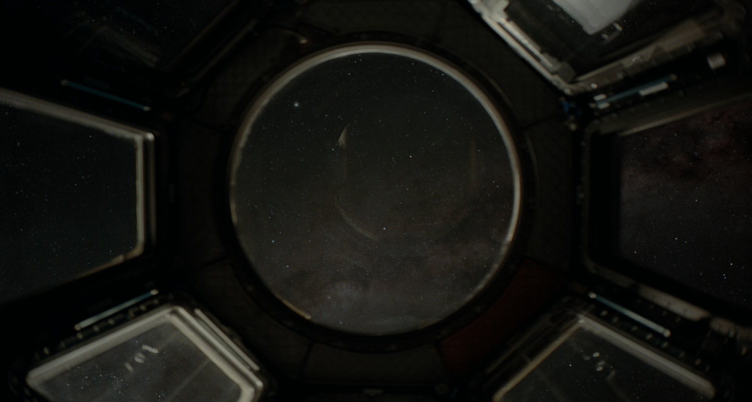

 M53, a globular cluster in the Coma Berenices constellation. These dense clusters of stars are some of the oldest objects in the universe. (credit)
 The Iris Nebula in Cepheus, a region of the vast galactic Integrated Flux Nebula that sits above our position on the galactic plane. This region of space is illuminated by the blazing light of a blue star. (credit)
 I took this image on a backpacking trip in Utah in early Summer. The seeing that night was good enough to see detail in the dust lanes in the Milky Way and for this one minute exposure to reveal the golden color and even the Lagoon, Trifid, and Eagle nebulae looking into the core of our galaxy.
 This image comes from the City of Rocks in Idaho, a beautiful natural preserve where you can go to appreciate the night sky unimpeded by the light pollution of large cities. To the right of the core of the Milky Way you can see the Rho Ophiuchi Cloud Complex containing the intensely orange star Antares and a region of dark dust that will show up even with phone photography.


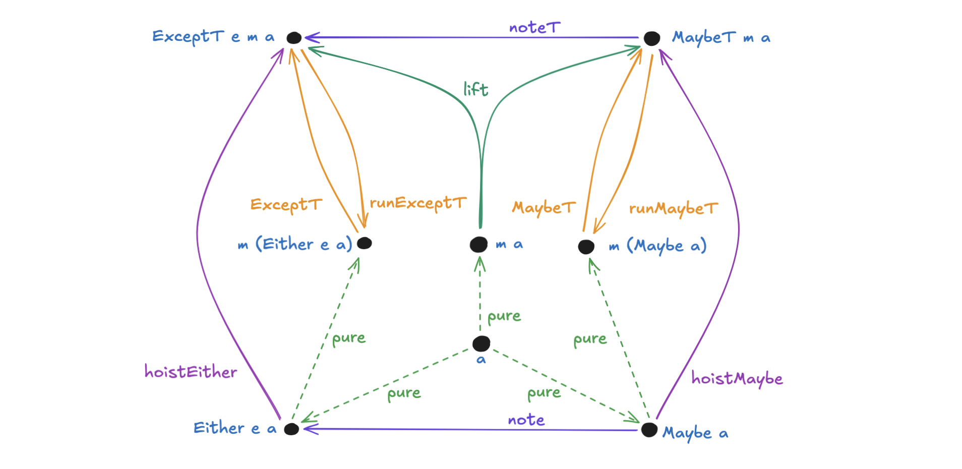


 Artwork by my good friend
  Hydrogen wave function solutions (
 The Riemann Zeta Function, graphed (
 A small sample of connected concepts in algebraic regions of mathematics.
 An eigen-operator Q acting on an object Psi yields Psi again, but scaled by a factor of q.
 Dominoes (
 λ-2D: An artistic Lambda Calculus visual language (from
  The Y Combinator expressed in John Tromp’s
  The Lambda Cube, where → indicates adding dependent types, ↑ indicates adding polymorphism, and ↗ indicates allowing type operators.) (
 Haskell’s logo combines the lambda with a symbol ⤜ representing monadic binding.
 Ripples on an alpine lake.
 Cantor’s Diagonal Argument from Max Cooper’s
 A diagram conveying the Categorical Product.
 Artwork by my good friend Sophia Wood


 Figure from


